Descriptive Statistics
Getting set up
Ensure you have the PISA 2022 data frame loaded. If you can see the PISA_2022 data frame in your environment window (at the top right of your screen), there is no need to reload.
1 Descriptive statistics
1.1 The PISA assessments
The first International Large-Scale Assessment (ILSA) comparing the learning outcomes of school students between countries was attempted in the 1960s. However, ILSAs only became established and regular in the late 1990s and 2000s.
The OECD’s Programme for International Student Assessment (PISA) has tested 15-year-old students in a range of “literacies” or “competencies” every three years since 2000. There is a rotating focus on reading, mathematics and science, with PISA 2021 focusing on mathematics but delayed by the global pandemic until 2022 and the results only published in December 2023. Until then, PISA 2018, with a focus on reading, was the most recently available cycle and PISA 2015 remains the most recent cycle focusing on science.
In addition to reading, mathematics and science, PISA has tested students on a range of “novel” competencies including problem-solving, global competence, financial literacy, and creative thinking. In addition to these tests, PISA also administers questionnaires to students, teachers and parents to identify “factors” which explain test score differences within and between countries.
Since 2000, more than 90 “countries and economies” and around 3,000,000 students have participated in PISA. The growth in the number of countries participating in each cycle of PISA is reflected in the growth in the number of students taking the PISA tests and responding to the PISA questionnaires, as shown in Table 1.
Table 1: Number of students participating in PISA by year
| Year | Number completing assessment |
|---|---|
| 2000 | 265,000 |
| 2003 | 275,000 |
| 2006 | 400,000 |
| 2009 | 470,000 |
| 2012 | 510,000 |
| 2015 | 540,000 |
| 2018 | 600,000 |
| 2022 | 690,000 |
There is a degree of inherent error in all educational and psychological assessments - and indeed in all social or physical measurement. ILSAs such as PISA may be more prone to error because their comparisons across large and diverse populations make them particularly complex. However, it is particularly important to minimise the error in ILSAs because they influence education policy and practice across a large number of education systems, impacting a vast population of students beyond those sampled for the assessments.
According to the OECD (2019), three sources of error are worth considering. First, sampling error, uncertainty in the degree to which results from the sample generalise to the wider population - in 2018, the OECD average sampling error was 0.4 of a PISA point score (the value was not reported for 2022). Second, measurement error, uncertainty in the extent to which test items measure proficiency. In 2018, the measurement error was around 0.8 of a point in mathematics and science and 0.5 of a score point in reading (the measurement error was not reported for 2022). Third, the link error is the uncertainty in comparison between scores in different years. For comparisons of science scores between 2018 and 2015, the link error is 1.5 points. For 2018-2022, the link errors are reading (1.47), mathematics (2.24) and science (1.61) (OECD 2022, 293)
PISA uses a probabilistic, stratified clustered survey design (Jerrim et al. 2017). However, sampling issues including sample representativeness, non-response rates and population coverage have been identified (Zieger et al. 2022; Rutkowski and Rutkowski 2016; Gillis, Polesel, and Wu 2016; Hopmann, Brinek, and Retzl 2007). Furthermore, Anders et al. (2021) and Jerrim (2021) have shown that assumptions for imputing values (imputing means estimating any missing values based on existing data - for example by adding a mean or mode score for a missing test) for non-participating students used to construct the sample may have significant impacts on achievement scores.
Since PISA 2015, the majority of participating countries have switched from paper-based assessment to computer-based assessment (Jerrim 2016). A randomised controlled trial conducted by the OECD prior to the switch indicated a difference in score between the two modes of delivery. The OECD introduced an adjustment to compensate for this difference, but it is not entirely removed by the adjustment Jerrim et al. (2018), with implications for any time series comparisons between PISA cycles. Nonetheless, Jerrim (2016) notes that “in terms of cross-country rankings, there remains a high degree of consistency… the vast majority of countries are simply ‘shifted’ by a uniform amount” (pp. 508-509).
In summary, comparisons within and between countries and comparisons over time using ILSAs need careful interpretations that bear in mind the specific design of each ILSA. In practice, this means considering a range of potential explanations for score differences. Does a difference in science ranking between two countries simply reflect sampling error? Does the same parental occupation or home possessions amount to the same economic, social and cultural status in different countries (e.g. the social status of a parent as a teacher or the economic status of the number of cars a family owns)? Does a difference in mathematical self-efficacy (i.e. student self-confidence in mathematics) between the USA and Japan reflect sociocultural differences in self-enhancement and modesty, respectively? How do score differences between boys and girls indicate gender inequalities in education that reflect wider society?
For useful critique and discussion of the construction of the measure of socio-economic status in PISA data see: Avvisati’s (2020) paper.
1.2 Using the command line for descriptive statistics
For further reading on descriptive statistics see chapter 5 of Navaro’s Learning Statistics with R.
We are going to focus on the following variables in the PISA_2022 data frame:
CNT the country of the student.
HOMEPOS is a self-reported measure of a student’s wealth, linked to the number of possessions students report having in their home (e.g. books, computers, cars, phones etc.). It is a numeric variable, with a mean of -0.447, minimum of -10.07 and a maximum of 15.24.
ESCS is the index of economic, social and cultural status. It might be thought of as a measure of economic and social status (with some cultural capital measures included). It is a numeric variable, with a mean of -0.310, minimum of -6.84 and a maximum of 7.38. It is constructed from three items: highest parental occupation (
HISEI), highest level of parental education (PARED), and home possessions (HOMEPOS), including books in the homePV1MATH, PV1SCIE, PV1READ are the plausible value scores for achievement tests in mathematics, science and reading, respectively. The full achievement tests are long, so each student only completes a subset of items (which still takes 2 hours). Statistical models are then used to calculate an overall score, based on the students’ answers to the subset of questions, as if students had answered all the questions. Ten different approaches (ten different statistical models, that take different approaches to estimating the overalls score are used) to calculating a representative scores, plausible values are used, leading to ten different plausible values. In this course, will just use the first plausible value (PV1). This differs from the PISA recommendation for using the scores, but simplifies things for teaching. For more on plausible values see: What are plausible values?
ST004D01T is the gender variable and and can take the values:
Male,FemaleorNA.
The simplest way to find information about a data frame is to use the console. You can type commands to find out about a data frame directly into the console. To preform an action on a particular column (also called a vector), we use the $ symbol. For example, to refer to country data (which is in the vector CNT) we would use PISA_2022$CNT
In the command line, if you want to find the mean of all the repsonses to the HOMEPOS (Home Possessions, a proxy for wealth) item you can type the following:
mean(PISA_2022$HOMEPOS)
Notice that you get this response: [1] NA. An NA in the data frame can occur for a number of reasons, for example it may indicate a response is missing or incomplete, hence the mean can’t be calculated. To tell R to ignore NAs, we add na.rm = TRUE to a function:
mean(PISA_2022$HOMEPOS, na.rm = TRUE)
You can use the command line with a number of functions to find useful information about a data frame. R has a number of standard functions that might be useful for descriptive statistics. To find out details about data frames, you can use:
nrow()finds the number of rows (e.g.nrow(PISA_2022))ncol()finds the number of columns (e.g.ncol(PISA_2022))names()finds the names of all the columns (e.g.names(PISA_2022))
If you are working on individual columns, e.g. max(PISA_2022$PV1SCIE), you can use:
mean()- finds the arithmetic meanmedian()- finds the median valuemin()- finds the minimum valuemax()- finds the maximum valuesd()- finds the standard deviationrange()- finds the range of valueslength()- finds the number of itemsunique()- finds the unique items
Maybe surprisingly, there is no function to calculate the mode in the tidyverse package. However, you can get one by loading the modeest package and using the most frequent value (mfv) function.
# Install the modeest package to calculate a mode

library(modeest)
library(tidyverse)

# The mode can be found with the most frequent value (mfv) function
# We can look at about number of books in the home (ST255Q01JA)
# Then use mfv to find the mode value (note the na.rm=TRUE to avoid NAs)

mfv(PISA_2022$ST255Q01JA, na.rm = TRUE)
[1] 26-100 books
11 Levels: There are no books. 1-10 books 11-25 books ... No ResponseTo get a list of the item descriptors, you can use this code:
$CNT
[1] "Country code 3-character"

$CNTSCHID
[1] "Intl. School ID"

$CNTSTUID
[1] "Intl. Student ID"

$REGION
[1] "REGION"

$OECD
[1] "OECD country"

$LANGTEST_QQQ
[1] "Language of Questionnaire"

$ST003D02T
[1] "Student (Standardized) Birth - Month"

$ST003D03T
[1] "Student (Standardized) Birth -Year"

$ST004D01T
[1] "Student (Standardized) Gender"

$ST250Q01JA
[1] "Which of the following are in your [home]: A room of your own"

$ST250Q02JA
[1] "Which of the following are in your [home]: A computer (laptop, desktop, or tablet) that you can use for school work"

$ST250Q03JA
[1] "Which of the following are in your [home]: Educational Software or Apps"

$ST250Q05JA
[1] "Which of the following are in your [home]: Internet access (e.g. Wi-fi) (excluding through smartphones)"

$ST251Q01JA
[1] "How many of these items are there at your [home]: Cars, vans, or trucks"

$ST251Q06JA
[1] "How many of these items are there at your [home]: Musical instruments (e.g. guitar, piano, [country-specific example])"

$ST251Q07JA
[1] "How many of these items are there at your [home]: Works of art (e.g. paintings, sculptures, [country-specific example])"

$ST253Q01JA
[1] "How many [digital devices] with screens are there in your [home]?"

$ST254Q01JA
[1] "How many of the following [digital devices] are in your [home]: Televisions"

$ST254Q02JA
[1] "How many of the following [digital devices] are in your [home]: Desktop computers"

$ST254Q03JA
[1] "How many of the following [digital devices] are in your [home]: Laptop computers or notebooks"

$ST254Q04JA
[1] "How many of the following [digital devices] are in your [home]: Tablets (e.g. [iPad®], [BlackBerry® Playbook™])"

$ST254Q05JA
[1] "How many of the following [digital devices] are in your [home]: E-book readers (e.g. [Kindle™], [Kobo], [Bookeen])"

$ST254Q06JA
[1] "How many of the following [digital devices] are in your [home]: [Cell phones] with Internet access (i.e. smartphones)"

$ST255Q01JA
[1] "How many books are there in your [home]?"

$ST256Q02JA
[1] "How many of these books at [home]: Classical literature (e.g. [Shakespeare], [Example 2])"

$ST005Q01JA
[1] "What is the [highest level of schooling] completed by your mother?"

$ST007Q01JA
[1] "What is the [highest level of schooling] completed by your father?"

$ST019AQ01T
[1] "In what country were you and your parents born? You"

$ST019BQ01T
[1] "In what country were you and your parents born? Mother"

$ST019CQ01T
[1] "In what country were you and your parents born? Father"

$ST125Q01NA
[1] "How old were you when you started [ISCED 0]: Years"

$ST261Q01JA
[1] "Why miss school for 3+ months: I was bored."

$ST261Q04JA
[1] "Why miss school for 3+ months: I could not reach school because of transportation problems."

$ST062Q02TA
[1] "In the last two full weeks of school, how often: I [skipped] some classes"

$ST038Q08NA
[1] "In past 12 months, how often: Other students spread nasty rumours about me."

$ST016Q01NA
[1] "Overall, how satisfied are you with your life as a whole these days?"

$ST337Q07JA
[1] "In your school, how often participate in: Science [club]"

$ST324Q11JA
[1] "Agree/disagree: School has been a waste of time."

$ST355Q03JA
[1] "Confident can do in future: : Finding learning resources online on my own"

$FL150Q02TA
[1] "Have you learned to manage money in a course: At school as part of another subject or course"

 [ reached getOption("max.print") -- omitted 44 entries ]
Alternatively, you can read a complete list of the items in PISA here: PISA 2022 student survey item descriptors
A useful way to get a quick summary of what is in a data.frame is, the summary command. This command outputs the minimum, median, mean, maximum (and 1st and 3rd quartile values, i.e. the values at 25% and 75% of the range). For example, to get a sense of the science score variable (PV1SCIE) we can use:
2 Filtering Data frames
We will now learn how to calculate means of subgroups of data frames, using the filter and summarise functions. We can use filter to focus on only a subset of our data.frame. For example, below, we can use filter to focus only on responses from UK students.
Note, in R the = and == operators have slightly different meanings. = can be used to assign a value, for example to set x to 10.
By contrast, when checking is two items are equal, use ==
In line 4 below, we filter for UK responses. Note that, in filter we use == rather than =.
Then we use summarise to calculate the means of the variables we are interested in, for example, students science (PV1SCIE), mathematics (PV1MATH) and reading scores. We can also find the total number of students entered in the UK, using n(), which counts the number of rows.
- 1
-
line 1 passes the whole
PISA_2022dataset and pipes it into the next line using%>% - 2
-
line 2
filtersout any results that are not from the UK by finding all the rows whereCNTequals=="United Kingdom". Note the==for checking equality. The result is then piped (%>%) to the next line - 3
-
line 3 uses
summariseto calculate, for the UK, the mean ofPV1SCIE(the science score) and puts the result in a column calledMeanSci - 4
-
line 4 uses
summariseto calculate, for the UK, the mean ofPV1MATH(the maths score) and puts the result in a column calledMeanMath - 5
-
line 5 uses the
n()function to count the number of students in the UK sample
# A tibble: 1 × 3
  MeanSci MeanMath Total
    <dbl>    <dbl> <int>
1 492. 483. 12972If you want to filter by a different vector (that is, a different column in the table), don’t forget to change the name of the vector in the filter command, for example, to find the mean mathematics and science scores, and total number of pupils who are girls (using the gender variable ST004D01T). We change the vector to filer on to ST004D01T and the condition to Female.
Don’t forget to use the %>% and the == in filter!
# A tibble: 1 × 3
  MeanSci MeanMath  Total
    <dbl>    <dbl>  <int>
1    452.     438. 305759
You can add multiple filters by using the & operator which means AND. Later on we will also meet | (the vertical line symbol), which means OR. So if you want to find the scores of male students in the UK you would use:
Often we are interested in summary data across multiple subgroups. We can then tell R to group_by, for example, group_by(CNT), to get a summary of data for subgroups.
- 1
-
line 1 passes the whole
PISA_2022dataset and pipes it into the next line using%>% - 2
-
line 2 uses
group_byto use the values inCNTto group the data - i.e. the calculate the means for each country - 3
-
line 3 uses
summariseto calculate the mean ofPV1SCIE(the science score) and puts the result in a column calledMeanSci - 4
-
line 4 uses
summariseto calculate the mean ofPV1MATH(the maths score) and puts the result in a column calledMeanMath - 5
-
line 5 uses the
n()function to count the number of students the sample
# A tibble: 80 × 4
   CNT                  MeanSci MeanMath Total
   <fct>                  <dbl>    <dbl> <int>
 1 Albania                 376.     368.  6129
 2 United Arab Emirates    436.     434. 24600
 3 Argentina               415.     389. 12111
 4 Australia               508.     487. 13437
 5 Austria                 494.     491.  6151
 6 Belgium                 495.     494.  8286
 7 Bulgaria                422.     418.  6107
 8 Brazil                  406.     380. 10798
 9 Brunei Darussalam       445.     440.  5576
10 Canada                  499.     484. 23073
# ℹ 70 more rowsIn the console, R will truncate tables, so you might only see the first 10 countries of 80 in the data frame using the code above. One solution to this is to put the results of the summarising into a new data frame (e.g. summarydata) which you can then view from the environment window (and use for future processing). To do this you use the assign operator <-.
3 Creating summary tables and manipulating them
The PISA data frame is large (!) so it can often be helpful to create interim summary tables.
When using summarise, be careful to add a comma after each function, and check you have closed as many brackets as you open!
A useful function is table which creates a summary table of the counts of unique entries in a data frame. For example, we might want to know how many boys and girls there are by country in the whole data set.
In the example below, we will use select which creates a subset of a table by columns. For example, if I want to create a table of gender type by country, we need only include two columns from the PISA_2022 data frame: country (CNT) and gender (ST004D01T). We use the command select to focus on those two: select(CNT, ST004D01T).
To create a summary table, intuitively, we use the table function. There are two additional actions we need to do. First, because we piped the whole PISA_2022 data frame, if we apply table, then even though we have filtered by the UK, the data frame retains levels for all the other countries. If we don’t remove these levels, we will get a large data frame with many zero entries for the countries we have filtered out. The function droplevels() removes the levels for other countries (i.e. everything other than the United Kingdom). Finally, the output of table is a datatype called (appropriately) a table. Data frames are more easily manipulated so we convert the table into a data frame using as.data.frame(table(SchoolType)).
- 1
-
line 1 creates a new data frame,
GenderUKinto which the results manipulatedPISA_2022will be placed -PISA_2022is piped to the next steps - 2
-
line 2 uses
selectto select the columns of interestCNT(country) andST004D01T(gender) - 3
-
line 3 uses
filterto filter for only the entries for the UK - 4
-
line 4 - as we have filtered for the UK, we would get 0 entires for all the other levels (all the other countries). To stop those 0s confusing our table we use
droplevels()to ignore the levels we don’t need - 5
-
line 5 - to create summary of the counts, we use
tableto create a summary table. We turn the table into a data frame withas.data.frameto make it easier to manipulate - 6
- line 6 - print the table
             CNT ST004D01T Freq
1 United Kingdom    Female 6397
2 United Kingdom      Male 6575
You can open the GenderUKSummary data frame and see the summary data. Table has created a new column Freq which stores the results of the counts.
It might now be interesting to know what percentage the counts of genders represent. To achieve that, first we create a variable that is the total number of genders (to calculate the percentage). This variable is total, and we perform a simple sum on the count column - GenderUKSummary$Freq.
We then use the mutate function. mutate allows you to add a new column to a table. You pipe the data frame to mutate, and begin by giving the name of the new column you want, in this case the percentage of schools of each type, we will call this PerSch mutate(PerSch=. Then we set the value of that column to the percentage calculation: 100*(Freq/total). The Frequency count for each column will be multiplied by 100 and divided by the total.
- 1
-
line 1 - to calculate a percentage, you first need to find the total of the frequency column in
GenderUKSummary. We useGenderUKSummary$Freqto indicate the column andsumto find the total
- 2
-
line 2 - pipe
GenderUKSummaryso we can manipulate it - 3
-
line 3 - to add a new column (with the percentage in) we use
mutate. We give the name of the new columnPerSch =and set out the calculation we want to perform, dividing the frequency in each row, by the total and multiplying by 100:100*(Freq / total)
             CNT ST004D01T Freq   PerSch
1 United Kingdom    Female 6397 49.31391
2 United Kingdom      Male 6575 50.68609
We can also get the same result by using the sum function inside mutate. Here PerSch is calculated for each row, taking the Freq value for that row and dividing it by the sum of Freq for all rows, i.e. calculating the percentage:
You can use the round function to display a given number of decimal places. Here, I have used round( ,2) to limit the percentage calculation to two significant figures.
4 Seminar activities
4.1 Task 1 - Using the command line
- Using the command line, find out:
- The number of students (i.e. the number of rows) in the PISA 2022 data frame
- The number of items in our data frame (i.e. the number of columns)
- The mean, maximum and minimum science score (don’t forget to use
$) - The unique values of
ST003D02T- what information do you think this column holds?
Answer
# Using the command line
# a) Find the number of students (i.e. the number of rows) in the PISA 2022 data frame

nrow(PISA_2022)

# b) The number of items in our data frame (i.e. the number of columns)

ncol(PISA_2022)

# c) The mean, maximum and minimum science score (don't forget to use $)

mean(PISA_2022$PV1SCIE)
max(PISA_2022$PV1SCIE)
min(PISA_2022$PV1SCIE)

# d) The unique values of ST003D02T - what information do you think this column holds?

unique(PISA_2022$ST003D02T)

# This column contains students' birth months
# You can find out the subtitle of columns using

attributes(PISA_2022$ST003D02T)
4.2 Task 2 - Using the summary function
- Using
summaryfind:
- The maximum and minimum of the HOMEPOS (Wealth) variable
- The mean reading score
- The minimum science score in the data set
- Consider the distributions of the reading and science scores, and comment on any differences.
4.3 Task 3 - Creating summary tables
Make sure you have spelled the name of the variables PV1MATH, etc. correctly. They are case sensitive. You can use the function colnames(PISA_2022) to get a list of names and copy and paste them.
Find the total number of students who responded in the United States, and their mean science, mathematics and reading scores. Compare that to the responses from the UK. Don’t forget to pipe (
%>%) each step!Filter the data frame for the UK and
group_bygender (which isST004D01T). Use summarise to find the maximum, minimum and mean scores for boys and girls in mathematics in the UK.Filter the data frame for the UK, the US, and
group_bygender (which isST004D01T) and country. Use summarise to compare mathematics and science achievement.
Answer
# Summarising responses in the US and UK and finding means

PISA_2022 %>%
 filter(CNT == "United Kingdom" | CNT == "United States")%>%
  group_by(CNT)%>%
  summarise(MeanSci = mean(PV1SCIE),
            MeanMath = mean(PV1MATH),
            MeanRead = mean(PV1READ),
            Total = n())

# Comparing male and female mathematics performance in the UK

PISA_2022 %>%
 filter(CNT == "United Kingdom")%>%
  group_by(ST004D01T)%>%
  summarise(MeanUKMath = mean(PV1MATH),
            MaxUKMath = max(PV1MATH),
            MinUKMath = min(PV1MATH))

# Comparing male and female mathematics performance in the UK and US

PISA_2022 %>%
  filter(CNT == "United Kingdom" | CNT== "United States" )%>%
  group_by(ST004D01T, CNT)%>%
  summarise(MeanMath = mean(PV1MATH),
            MaxMath = max(PV1MATH),
MinMath = min(PV1MATH))Don’t forget to use the pipe operator %>% between each function!
WB171Q01HA asks participants to think of the last time you had a break between classes at school: How did you feel: Happy. For students in France, find out the percentage of students who responded with the different options: Not at all A little Quite a bit Extremely Valid Skip Not Applicable Invalid No Response Missing. (Hint: don’t forget to droplevels()).
Answer
# Finding the percentage of students who feel happy between lessons in France

WellData<-PISA_2022%>%
  select(CNT, WB171Q01HA)%>%
  filter(CNT == "France")%>%
  droplevels()

WellData<-as.data.frame(table(WellData))
Total = sum(WellData$Freq)
WellData<-WellData%>%
  mutate(WellData=round((Freq*100 / Total),1))

WellData
ST251Q06JA asks students if they have a musical instrument in their home. What percentage of students in the UK have no instruments in their home? What is the percentage in Korea?
Answer
# Finding the percentage of students with no musical instruments in the UK and Korea
# Select the relevant variables, filter for the countries and group - dropping levels to cut unnecessary countries
MusicData <- PISA_2022%>%
  select(CNT, ST251Q06JA)%>%
  filter(CNT == "United Kingdom"|CNT == "Korea")%>%
  group_by(ST251Q06JA, CNT)%>%
  droplevels()

# Convert to a data frame

MusicData<-as.data.frame(table(MusicData))

# Find the total number of students to calculate percentages
Total = sum(MusicData$Freq)

# Mutate to add a column with the percentage calculation
MusicData<-MusicData%>%
  mutate(PercComp = round((Freq*100 / Total), 1))

MusicDataDon’t forget to use the pipe operator %>% between each function!
4.4 Categorising data
A useful analytical choice is to categorise some a numerical variable into ordinal classes. For example, rather than treating HOMEPOS as a continuous scale, you might want to split into high and low wealth groups (for example, those above and below the mean value).
To do this, first calculate the mean mean(HOMEPOS). Then we add a new vector, which we will call wealthclass using the mutate function. We set the value of wealthclass using ifelse. If HOMEPOS is more than the mean score, we set wealthclass to High, and if it is anything else, we set it to Low. We do that using wealthclass = ifelse(HOMEPOS > MeanUKwealth, "High", "Low"). Note, in ifelse, the first value is returned if the identity is true (i.e. if HOMEPOS > MeanUKwealth wealthclass is set to High). If the value if not true, the second value is set (e.g. if HOMEPOS is not > MeanUKwealth then wealthclass is set to LOW).
For example, create a data frame of UK participants HOMEPOS sorted into HIGH and LOW categories.
# Create a data frame of UK responses
UKPISA2022 <- PISA_2022 %>%
  select(CNT, HOMEPOS) %>%
  filter(CNT == "United Kingdom") %>%
4  mutate(wealthclass =  ifelse(HOMEPOS > mean(HOMEPOS, na.rm=TRUE),
                               "High",
                               "Low"))
UKPISA2022- 4
-
line 4 - mutate to create a new column
wealthclass- if HOMEPOS is more than mean(HOMEPOS), set the column to “High” otherwise set it to “Low”
# A tibble: 12,972 × 3
   CNT            HOMEPOS wealthclass
   <fct>            <dbl> <chr>
 1 United Kingdom  -1.09  Low
 2 United Kingdom  -0.418 Low
 3 United Kingdom   1.13  High
 4 United Kingdom  -0.829 Low
 5 United Kingdom  -0.274 Low
 6 United Kingdom  NA     <NA>
 7 United Kingdom  -0.606 Low
 8 United Kingdom  NA     <NA>
 9 United Kingdom   0.425 High
10 United Kingdom   0.998 High
# ℹ 12,962 more rows
4.5 Seminar activities
4.5.1 Task 1 Create a ranked list
Create a ranked list of countries by their mean science scores (PV1SCIE). What are the top five countries for science? Do the same for wealth (HOMEPOS). What patterns do you notice? Why might a researcher be critical of such rankings [Extension: Include the standard deviation of each country (hint: use the sd function) - can you detect any patterns?]
Note that the PISA 2022 links wealth to HOMEPOS (a self reported measure of possessions in the home). You might want to consider the implications of that definition for interpreting the data
Show the answer
# Create a ranked data data frame for science

PISA2022SciRank <- PISA_2022 %>%
  select(CNT, PV1SCIE) %>% # Select variables of interest
  group_by(CNT) %>% # group by country
  summarise(meansci = mean(PV1SCIE)) %>%
     # summarise  country data to find the mean Sci score
  arrange(desc(meansci)) # arrange in descending order based on the meansci score

print(PISA2022SciRank)
# A tibble: 80 × 2
CNT meansci
<fct> <dbl>
1 Singapore 561.
2 Japan 546.
3 Macao (China) 543.
4 Korea 531.
5 Estonia 527.
6 Chinese Taipei 527.
7 Hong Kong (China) 525.
8 Czech Republic 511.
9 Australia 508.
10 Poland 505.
# ℹ 70 more rowsShow the answer
# And repeat the ranking for wealth

PISA2022WealthRank <- PISA_2022 %>%
  select(CNT, HOMEPOS) %>% # Select variables of interest
  group_by(CNT) %>% # group by country
  summarise(meanwel = mean(HOMEPOS, na.rm=TRUE)) %>%
     # summarise  country data to find the mean Sci score
  arrange(desc(meanwel)) # arrange in descending order based on the meansci score

print(PISA2022WealthRank)
# A tibble: 80 × 2
CNT meanwel
<fct> <dbl>
1 Norway 0.547
2 Australia 0.483
3 Korea 0.371
4 New Zealand 0.367
5 Canada 0.348
6 Iceland 0.346
7 Sweden 0.327
8 Ireland 0.318
9 Malta 0.308
10 Austria 0.280
# ℹ 70 more rowsShow the answer
# With standard deviations

PISA2022SciRank <- PISA_2022 %>%
  select(CNT, PV1SCIE) %>% # Select variables of interest
  group_by(CNT) %>% # group by country
  summarise(meansci = mean(PV1SCIE),
            sdsci = sd(PV1SCIE)) %>%
  # summarise  country data to find the mean Sci score
  arrange(desc(meansci)) # arrange in descending order based on the meansci score

print(PISA2022SciRank)
# A tibble: 80 × 3
CNT meansci sdsci
<fct> <dbl> <dbl>
1 Singapore 561. 99.6
2 Japan 546. 92.7
3 Macao (China) 543. 86.6
4 Korea 531. 104.
5 Estonia 527. 87.7
6 Chinese Taipei 527. 102.
7 Hong Kong (China) 525. 91.1
8 Czech Republic 511. 103.
9 Australia 508. 107.
10 Poland 505. 94.2
# ℹ 70 more rowsShow the answer
PISA2022WealthRank <- PISA_2022%>%
  select(CNT, HOMEPOS)%>% # Select variables of interest
  group_by(CNT) %>% # group by country
  summarise(meanwel = mean(HOMEPOS, na.rm=TRUE),
            sdwel = sd(HOMEPOS, na.rm=TRUE)) %>%
  # summarise  country data to find  mean wealth score
  arrange(desc(meanwel))
  # arrange in descending order based on the meanwel score
print(PISA2022WealthRank)
# A tibble: 80 × 3
CNT meanwel sdwel
<fct> <dbl> <dbl>
1 Norway 0.547 0.970
2 Australia 0.483 0.861
3 Korea 0.371 1.01
4 New Zealand 0.367 0.862
5 Canada 0.348 0.867
6 Iceland 0.346 0.805
7 Sweden 0.327 0.878
8 Ireland 0.318 0.818
9 Malta 0.308 0.857
10 Austria 0.280 0.938
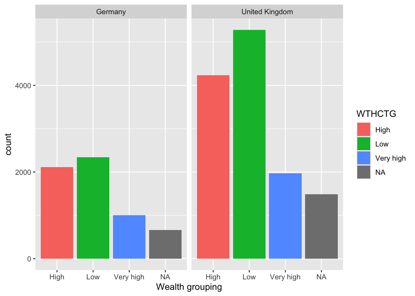
# ℹ 70 more rows4.5.2 Task 2 Categorise HOMEPOS scores
Categorising Variables
Split the HOMEPOS variable for the UK and Germany into the following groups:
| HOMEPOS | Name of category |
|---|---|
| >1 | Very High |
| 0>HOMEPOS<1 | High |
| 0< | Low |
Plot bar graphs of participants in these categories for both countries.
• What differences can you observe between the countries?
Hint: You can use mutate with if_else to do the categorisation. For more than two categories, you can use nested ifelses. In the example below, if the math score is more than 400, you go to the second ifelse to check if it is over 500. If both ifelses (over 400 and over 500) are met, the score is categorised as “Very High”. If the score is between 400 and 500, the first ifelse is met, but not the second, so the else condition of the second is met and the score set to “High”. If neither condition is met, the MATHSCORECAT is set to “Low”.
Show the answer
# Create a data frame for the UK and Germany
# Mutate the WTHCTG (wealth category) column by the boundaries of wealth categories
Wealth <- PISA_2022 %>%
  select(CNT, HOMEPOS) %>%
  filter(CNT == "United Kingdom" | CNT == "Germany") %>%
  mutate(WTHCTG = ifelse(HOMEPOS > 0,
                       ifelse(HOMEPOS > 1,
                             "Very high",
                             "High"),
                       "Low"))%>%
  group_by(CNT) %>%
  droplevels()

ggplot(data = Wealth,
       aes(x = WTHCTG, fill = WTHCTG))+
  geom_bar()+
  facet_wrap(.~CNT)+
  xlab("Wealth grouping")