If you have not taken the Introduction to R course, you should ccomplete the self-assessment questions below to ensure you are at the same level as those you have taken the Introduction course. If you have taken the course, you can skip this section. Using generative AI tools such as ChatGPT to complete the tasks indicates that you do not have sufficient knowledge of R to complete the intermediate course. You should complete the Introduction to R course before continuing with this course.
The questions require you to use the PISA_student_2022_subset.parquet dataset which you can download here here.
To load the PISA data:
Copy the following code and replace <folder> with the full folder location of where your dataset was saved, make sure that you have .parquet on the end. And keep the (r"[ ]")! Make sure you run all the lines in the code below, including the library(arrow) and library(tidyverse) lines.
examples of what this should look like for PC and Mac
# For Pete (PC) the address format was:PISA_2022 <-read_parquet(r"[C:\Users\Peter\KCL\MASTEMR\PISA_student_2022_subset.parquet]")# For Richard (Mac) the address format was:PISA_2022 <-read_parquet(r"[/Users/k1765032/Documents/Teaching/STEM MA/Quantitative module/Data sets/PISA_student_2022_subset.parquet]")
1.1 Question 1: Data manipulation
Produce a summary table of the mean science scores for countries in PISA 2022 for boys and girls
# A tibble: 165 × 3
# Groups:   CNT [80]
   CNT                  ST004D01T mean_sci
   <fct>                <fct>        <dbl>
 1 Albania              Female        390.
 2 Albania              Male          362.
 3 United Arab Emirates Female        445.
 4 United Arab Emirates Male          427.
 5 Argentina            Female        412.
 6 Argentina            Male          418.
 7 Australia            Female        507.
 8 Australia            Male          509.
 9 Australia            <NA>          566.
10 Austria              Female        489.
# ℹ 155 more rows
1.2 Question 2: Graphing
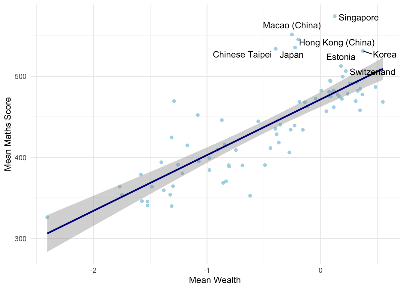
Plot a scatter plot of mean maths scores against mean wealth for the PISA countries. Add labels to countries with mean maths scores over 500, giving the name of the country. Add a linear regression line to the plot
Use a t-test to determine if male and female reading scores in the UK are statistically significantly different.
Use a chi-square test to determine if the number of boys and girls in the US and UK are diffrent
Show the code
# a) t-test# Filter the data for the UK and select relevant columnsuk_reading <- PISA_2022 %>%filter(CNT =="United Kingdom") %>%select(ST004D01T, PV1READ) %>%drop_na()# Perform the t-testt.test(PV1READ ~ ST004D01T, data = uk_reading)
    Welch Two Sample t-test

data:  PV1READ by ST004D01T
t = 10.159, df = 12960, p-value < 2.2e-16
alternative hypothesis: true difference in means between group Female and group Male is not equal to 0
95 percent confidence interval:
 15.03322 22.22110
sample estimates:
mean in group Female   mean in group Male
            500.2030             481.5759
Show the code
# p-value < 2.2e-16 so reject the null hypothesis there are statistically signifcant differences in mean reading scores in the UK# b) chi-square testUS_UK_gender <- PISA_2022 %>%filter(CNT %in%c("United States", "United Kingdom")) %>%select(CNT, ST004D01T) %>%droplevels()# Create a contingency tablecontingency_table <-xtabs(data = US_UK_gender, ~ ST004D01T + CNT)# Perform the chi-square testchisq.test(contingency_table)
    Pearson's Chi-squared test with Yates' continuity correction

data:  contingency_table
X-squared = 0.028622, df = 1, p-value = 0.8657
Show the code
# p-value = 0.8657 - p-value is over 0.05 so accept the null that the proportions of boys and girls in the UK and US is similar