Structural Equation Modelling (SEM) is an approach to representing the correlations between a number of variables linked to some phenomenon (Lomax 2013). A dependent variable (for example, scores on some test) might be linked to a number of independent variables (for example, hours of study, teacher’s level of experience, etc.). A powerful aspect of SEM is that it can be used to construct latent variables - variables which have explanatory usefulness but can’t be measured directly - out of a number of independent variables. Variables researchers can measure are called manifest variables, for example, mathematics, science and reading scores are manifest variables. These three scores might be taken to indicate intelligence, a latent variable, which can’t be measured directly.
To take another case, a researcher might wish to investigate how home environment impacts students’ mathematics achievement. There is no single variable, no single score, that can be measured to represent a young person’s home environment as 7/10 or 3/10. We might then consider their home environment a latent variable. We imagine that the nature of the circumstances in their home impacts their learning, but we cannot directly report the level of the home environment as a variable.
SEM allows us to propose a latent variable, like home environment, and calculate the contribution of a number of variables we can measure (e.g. the number of books in the home, parents’ occupation and level of education, family wealth, etc.) to the latent variable.
1.1 Assummptions of SEM
SEM is based on a number of assumptions:
Independence - the Observations are assumed to be independent of each other
No Perfect Multicollinearity - the independent variables are not perfectly correlated
Homoscedasticity - the variance of the residuals is constant
No multicollinearity - the independent variables are not highly correlated (Hoyle 2012)
Sample size - a large enough sample size to ensure the model is stable - assuming a common power level of 80% and significance levels of 0.05, and minimum path coefficient of 0.2, a sample size of 155 is required (Hair Jr et al. 2021)
1.2 Checks to carry out before fitting an SEM
Before fitting an SEM, it is important to check the data for a number of issues. These include:
Checking for multivariate normality - SEM assumes that the data is multivariate normally distributed. This can be checked using the mvn function in the MVN package.
# Create a subset of PISA data related to the UK containing the dependent variable of interest (PV1MATH) and the independent variables we are interested in1UKdata <- PISA_2022 %>%2select(CNT, PV1SCIE, PV1MATH, PV1READ) %>%3filter(CNT =="United Kingdom")# load the MVN package to check for multivariate normalitylibrary(MVN)# Check for multivariate normality using the Mardia test# note we drop the country and gender variable as they are not numeric and# omitting nas4mvn_result <-mvn(data = UKdata %>%select(-CNT) %>%na.omit())5mvn_result$multivariate_normality
1
line 1 passes the whole PISA_2022 dataset and pipes it into the next line using %>%
2
line 2 selects the variables of interest
3
line 3 filters for the UK
4
line 4 runs the test of multivariate normality removing the CNT column and omitting missing data
5
line 5 outputs the necessary statistics
           Test Statistic p.value     Method          MVN
1 Henze-Zirkler     2.587  <0.001 asymptotic ✗ Not normal
To interpret the output, look at the p-value of the Henze-Zirkler’s multivariate normality test. If the p-value is greater than 0.05, the data is considered to be multivariate normally distributed. If the p-value is less than 0.05, the data is not multivariate normally distributed.
You can also use qq plots to visually inspect the data for multivariate normality.
# Create QQ plots to visually inspect for multivariate normalitymultivariate_diagnostic_plot(data = UKdata %>%select(-CNT) %>%na.omit(),type ="qq")
The QQ plots show that the data does not follow a straight line, indicating that the data is not multivariate normally distributed.
In this case the assumption is not met. This might be due to the large sample size. If the sample size is large, the assumption of multivariate normality can be relaxed. However, if the sample size is small, it is important to check for multivariate normality. However, for a small sample, if the assumption is not met, a form of SEM estimation can be used which does not assume multivariate normality, such as the Weighted Least Squares Mean and Variance adjusted (WLSMV) estimator or the robust estimation method (MLR). These methods are discussed below.
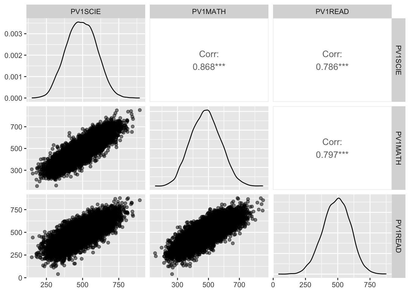
Checking for linearity - SEM assumes that the relationships between the variables are linear. This can be checked using scatterplots or correlation matrices. If the relationships are not linear, the data may need to be transformed or a different model may need to be used.
# Create a scatterplot matrix to check for linearitylibrary(GGally)1ggpairs(UKdata %>%select(PV1SCIE, PV1MATH, PV1READ),2lower =list(continuous =wrap("points", alpha =0.5)))
1
line 1 passes the UK data frame to the ggpairs function, selecting the variables of interest
2
line 2 specifies that the lower triangle of the scatterplot matrix should be plotted as points with some transparency (alpha = 0.5) to make it easier to see the density of points
There appear to be linear relationships between the variables PV1MATH, PV1READ and PV1SCIE, but there are some outliers.
No multicollinearity - SEM assumes that the independent variables are not highly correlated. This can be checked using the Variance Inflation Factor (VIF). A VIF value greater than 10 indicates high multicollinearity.
# Load the car package to check for multicollinearitylibrary(car)# Calculate the VIF for the independent variables1vif_values <-vif(lm(PV1MATH ~ PV1SCIE + PV1READ, data = UKdata))# Print the VIF valuesvif_values
1
line 1 fits a linear model to the data, using lm, with PV1MATH as the dependent variable and PV1SCIE and PV1READ as independent variables. This is like performing a test regression analysis to check for multicollinearity before performing the SEM.
 PV1SCIE  PV1READ
2.615497 2.615497
A VIF value greater than 10 indicates high multicollinearity. In this case, the VIF values for PV1SCIE and PV1READ are both less than 10, indicating that there is no high multicollinearity between the independent variables.
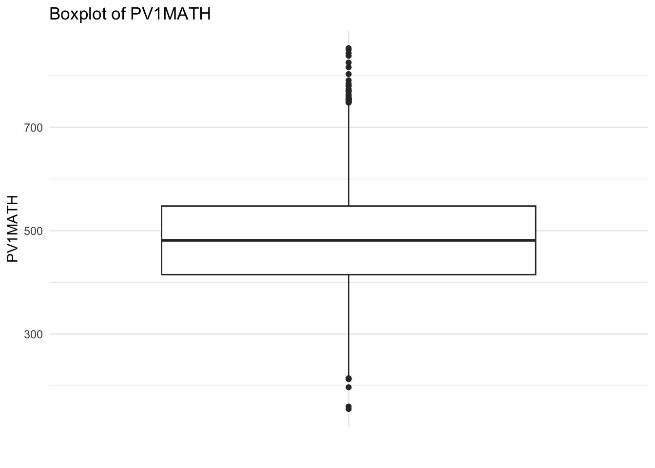
Checking for outliers - SEM is sensitive to outliers, so it is important to check for outliers before fitting the model. This can be done using boxplots or scatterplots. If there are outliers, they may need to be removed or transformed.
# Create boxplots to check for outliersggplot(UKdata, aes(x ="", y = PV1MATH)) +geom_boxplot() +labs(title ="Boxplot of PV1MATH", x ="", y ="PV1MATH") +theme_minimal()
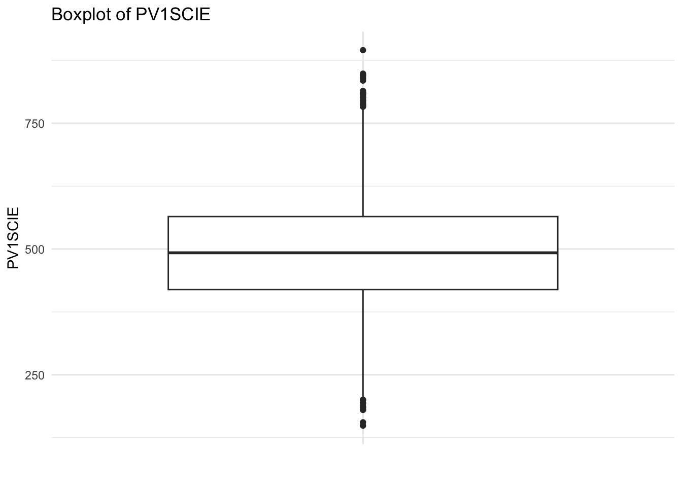
ggplot(UKdata, aes(x ="", y = PV1SCIE)) +geom_boxplot() +labs(title ="Boxplot of PV1SCIE", x ="", y ="PV1SCIE") +theme_minimal()
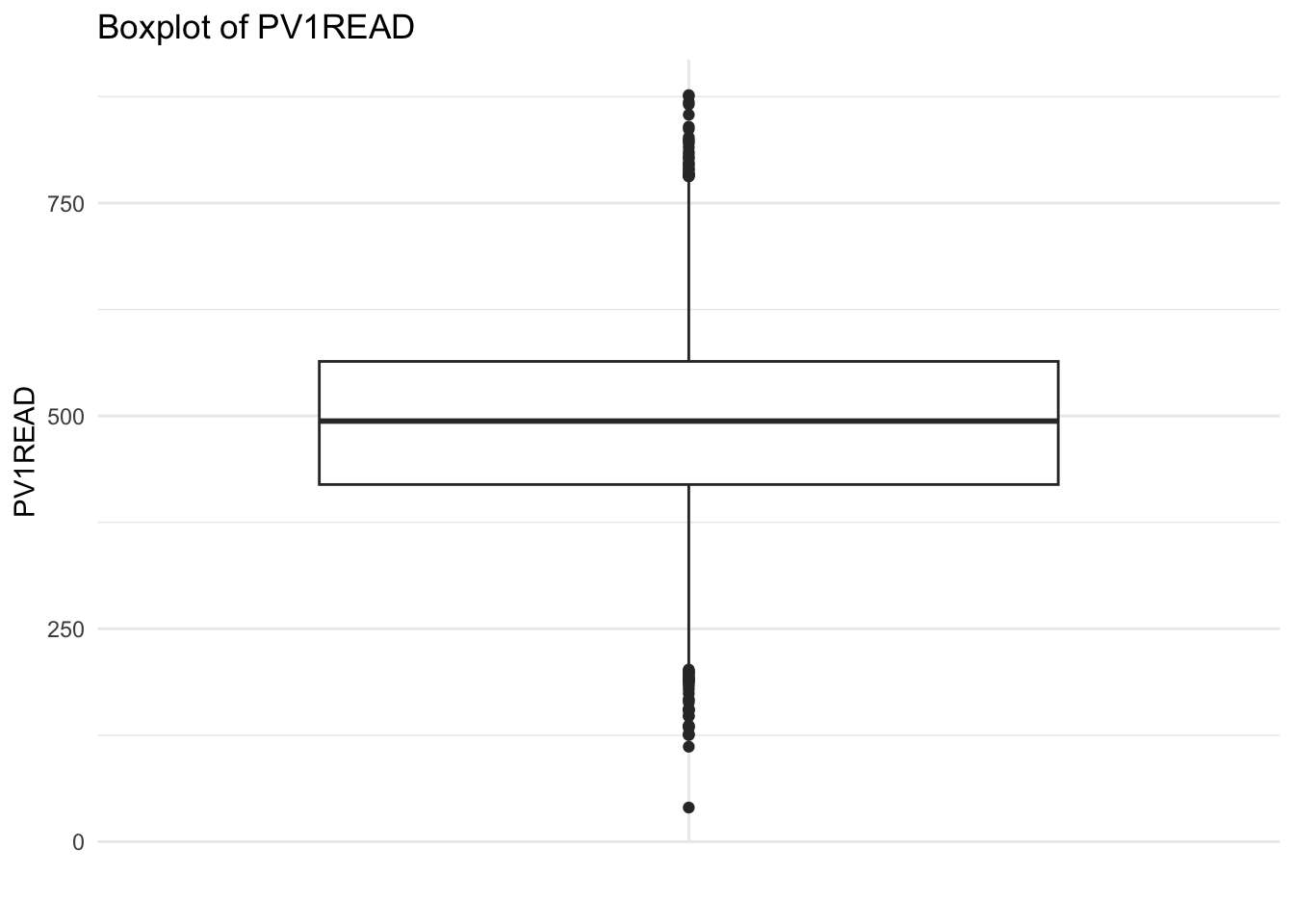
ggplot(UKdata, aes(x ="", y = PV1READ)) +geom_boxplot() +labs(title ="Boxplot of PV1READ", x ="", y ="PV1READ") +theme_minimal()
The boxplots show that there are some outliers in the data, particularly for PV1MATH and PV1SCIE. These outliers may need to be removed or transformed before fitting the SEM model.
One approach to dealing with outliers is to remove them from the data set. This can be done using the dplyr package in R. For example, to remove outliers from PV1MATH, we can use the filter function to keep only those values that are within 1.5 times the interquartile range (IQR) of the median.
line 1 uses the filter function to keep only those values of PV1MATH that are within 1.5 times the interquartile range (IQR) of the median.
This removes the outliers from the PV1MATH variable. The same process is used to remove outliers from the PV1SCIE variable.
Checking for missing data - SEM requires complete data, so it is important to check for missing data before fitting the model. This can be done using the mice package. If there is missing data, it may need to be imputed or removed.
# Load the `mice` package to check for missing datalibrary(mice)# Check for missing data using Little's MCAR testmd.pattern(UKdata)
 /\     /\
{  `---'  }
{  O   O  }
==>  V <==  No need for mice. This data set is completely observed.
 \  \|/  /
  `-----'
In this case there are no missing data. If data were missing, the mice package could be used to impute the missing data. Imputation is the process of replacing missing data with estimated values based on the observed data. The mice package provides a number of methods for imputing missing data, including predictive mean matching, Bayesian linear regression, and others. For example, the simplest approach to imputation is to replace all missing values with the mean of the variable.
An alternative to imputation using mice is to use Full Information Maximum Likelihood (FIML) estimation, which uses all available data to estimate the model parameters without imputing missing values. FIML is implemented in the lavaan package by setting the missing argument to "FIML" when fitting the model.
# Applying FIML estimation in lavaanmodel<-"PV1MATH ~ PV1SCIE + PV1READ + ESCS + HOMEPOS"fit <-sem(model, data = UKdata, missing ="FIML")
1.2.1 The steps to fitting an SEM model
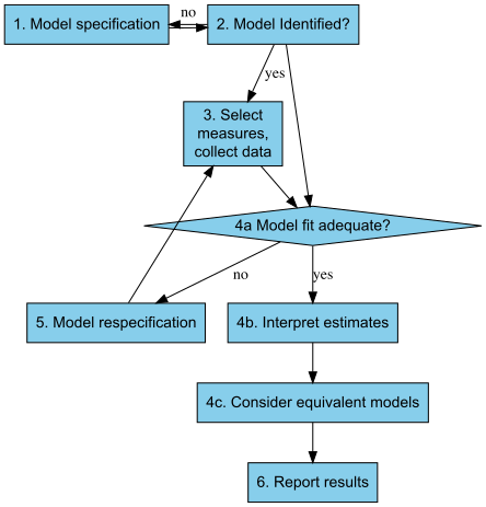
The typical steps taken when fitting an SEM model are shown below (see Figure 5.1 in (Kline 2023)):
Researchers typically begin by specifying a model, that is setting out the setting out the relationships theory suggest exists between variables. Specification is an important steps as the following stages assume the model is correct. model identification is the process of determining if a model can be estimated from available data. If the model is not identified, the researcher must go back to the model specification stage and make changes. If the model is identified, the researcher can move on to collecting data. Once data are collected, the model is estimated and the fit of the model is assessed (multiple approaches to assessing model fit are discussed below). If the model does not fit the data well, the researcher may need to respecify the model. If the model fits the data well, the researcher can interpret the estimates and consider equivalent models. For any model, there may be many (perhaps infintely many) other models that fit the data equally well.Finally, the researcher reports the results.
1.2.2 A simple structural model
Researchers use SEM to determine the correlations between a number of variable in a data set. It allows the relationship between multiple variables to be taken into account.
For example, in the PISA data set, in the context of data related to UK students achievement in mathematics, a researcher might be interested in building a model of mathematics (PV1MATH) score by a number of variables in the data set, for example, reading score (PV1READ), science score (PV1SCIE), family cultural capital (the index of economic, social and cultural status: ESCS), wealth (WEALTH) and gender (ST004D01T). SEM can be used to represent the relationship between these variables and students’ mathematics achievement.
To create the SEM we will use the lavaan package - lavaan is a contraction of Latent Variable Analysis and allows us to fit a number of different SEMs to data. We will also use the semPlot package to visualise the results. The relationships between variables in SEMs are often represented as path diagrams - representations in which variables are represented as squares or circles and arrows labelled with correlation coefficients join the variables to represent the relationships.semPlot allows us to draw path diagrams.
1.3 Model Syntax
Consider the SEM introduced above - a model of the variables that impact students’ mathematics scores.
To create the SEM of UK mathematics achievement we first create a subset data.frame of UK data, UKdata.
# Load lavaan to create the SEM and semPlot to draw path diagramslibrary(lavaan)library(semPlot)# Create a subset of PISA data related to the UK containing the dependent variable of interest (PV1MATH) and the independent variables we are interested in1UKdata <- PISA_2022 %>%2select(CNT, PV1SCIE, PV1MATH, PV1READ, ESCS, HOMEPOS, ST004D01T) %>%3filter(CNT =="United Kingdom")
1
line 1 passes the whole PISA_2022 dataset and pipes it into the next line using %>%
2
line 2 selects the variables of interest
3
line 3 filters for the UK
The first step is to create the model. Models in lavaan are represented as a dependent variable y, linked to a number of independent variables x1, x2, x3, etc. The ~ symbol is the regression operator. A simple regression formula might then take the form of:
y ~ x1 + x2 + x3
To indicate a variable is a latent variable we use the =~ operator. So to define a model in which the latent variable f1 varies with three independent variables we would write:
f1 =~ x1 + x2 + x3
In some cases, the independent variables may correlate. For example, if we are investigating mathematics achievement (the dependent variable, y), by looking at the independent variables of reading (x1) and science score (x2), it may be the case that reading and science cores covary (that is changes to one impacts the other). In this case, we can specify covariance in our model by stating:
y ~ x1 + x2 The regression model x1 ~ x2 Indicating the covariance
In our case, considering UK mathematics achievement, we can set up a model that mathematics score PV1MATH varies with science score PV1SCIE, reading score PV1READ, cultural resources in the home ESCS, a wealth proxy measure, HOMEPOS: model <- "PV1MATH ~ PV1SCIE + PV1READ + ESCS + HOMEPOS"
We then pass the model, and the data.frame to the sem function: fit<-sem(model, data=UKdata, estimator = "MLR"). This produces a model as the output fit. To see the results we call summary(fit)
Note that, as the data violated the check of multivariate normality above, we need to set the estimator to "MLR" (Maximum Likelihood with Robust standard errors). This estimator does not assume multivariate normality and is robust to violations of this assumption.
line 1 specify the model - we want to model PV1MATH using PV1SCIE, PV1READ, ESCS (class proxy) and HOMEPOS (wealth proxy).
2
line 2 create the model using the fit function
3
line 3 print the model
lavaan 0.6-20 ended normally after 1 iteration

  Estimator                                         ML
  Optimization method                           NLMINB
  Number of model parameters                         5

                                                  Used       Total
  Number of observations                         11083       12972

Model Test User Model:
                                              Standard      Scaled
  Test Statistic                                 0.000       0.000
  Degrees of freedom                                 0           0

Parameter Estimates:

  Standard errors                             Sandwich
  Information bread                           Observed
  Observed information based on                Hessian

Regressions:
                   Estimate   Std.Err  z-value  P(>|z|)
  PV1MATH ~
    PV1SCIE            0.565    0.007   82.056    0.000
    PV1READ            0.267    0.007   40.019    0.000
    ESCS               5.432    0.750    7.242    0.000
    HOMEPOS            1.027    0.715    1.436    0.151

Variances:
                   Estimate   Std.Err  z-value  P(>|z|)
   .PV1MATH         2006.033   28.472   70.456    0.000
In the regressions table, the function returns the value of the regression coefficients for each independent variable, and the P value (P(>|z|)). Note in the model above all the independent variables are significant, but the largest loading comes from the HOMEPOS (wealth) variable, with the science (PV1SCIE) and reading (PV1READ) scores contributing comparatively little.
Tip
In fitting a model, there are a number of approaches to estimating the model parameters. Different packages use different assumptions. To make your output match that of different SEM tools, you will need to choose the correct assumptions. For example, the default likelihood in lavaan is likelihood = "normal", which assumes multivariate normality. However, to match the output of AMOS, you would need to set the estimator to the default estimator = "ML" but the likelihood = "wishart". See the lavaan documentation for more details.
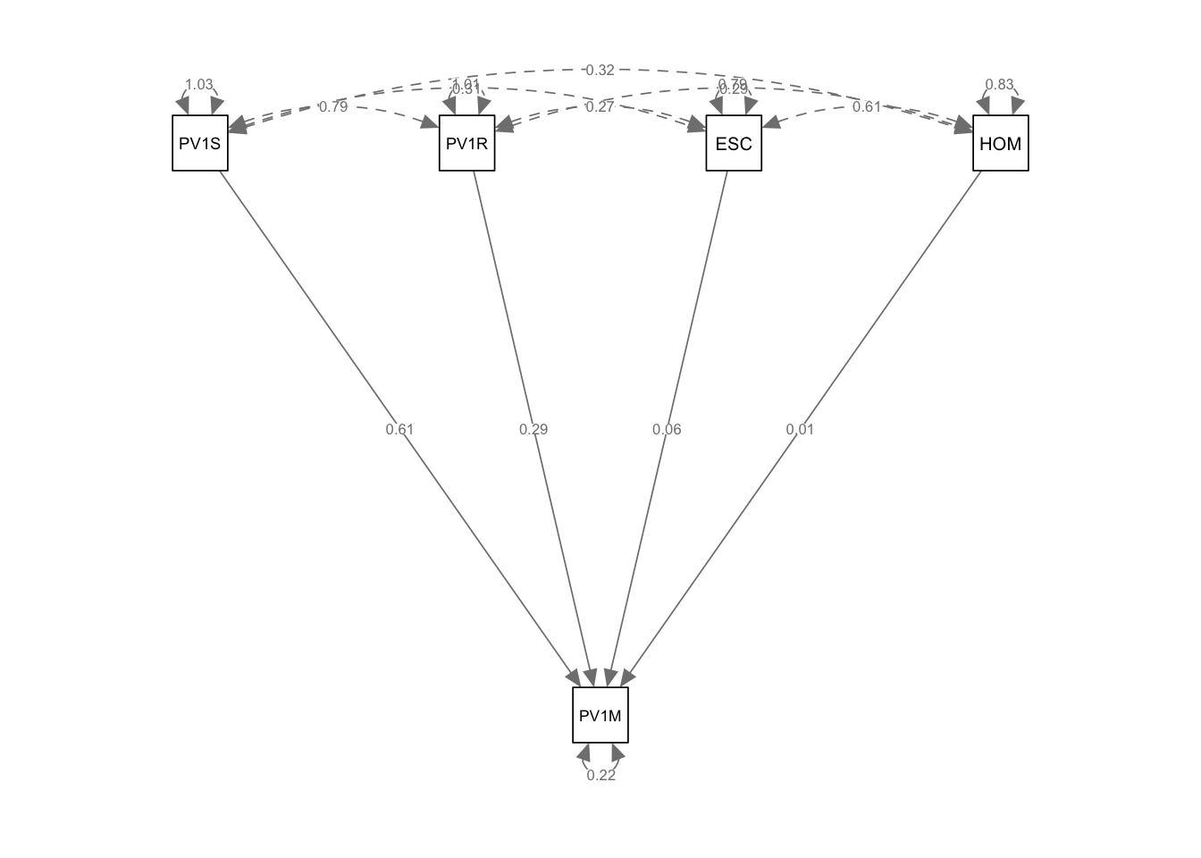
Finally, to produce a visual representation of the model, we pass our model, fit to the semPaths function (from the semPlot package we loaded above). We can specify was we want displayed on the lines, in this case the estimate of the regression coefficients between the variables.
In path diagrams, directly measured variables, manifest variables, are shown as squares. Latent variables are represented as circles. Single headed arrows represent the regression effects between variables. The curved arrows starting and ending on a square or circle indicate the variances of those variables. When curved arrows start and end on different variables, they represent covariance.
One issue to note here is the difference in the variance for the science and mathematics scores. PV1SCIE, PV1READ and PV1MATH are test scores and so have a large variance (the maximum and minimum science scores, for example, are 0 and 943). The variance of the two test variables is much greater that for HOMEPOS (Min=-10.0741 mean=-0.4447, Max=15.240) and ESCS (Min=-6.841 mean=-0.310, Max=7.380).
Tip
Continuous variables in data sets may have different ranges - that this the difference between the maximum and minimum variable can have larger magnitudes for some variables than others. This can be a problem because it can be hard to compare the effects of those variables. For example, in the PISA data, consider the difference between PV1MATH (mathematics scores) and HOMEPOS (a wealth proxy). The maximum and minimum mathematics scores are 155 and 893, while the maximum and minimum wealth scores are 8.2 and -6.8. The difference in the range of the variables can make it hard to compare the effects of the variables.
To compare the effects of the variables, we can normalise (also referred to as standardising, scaling or creating z scores) the variables. Normalising the variables sets the mean of the variable to 0 and the variance to 1. This makes the variables more comparable. The scale function in R can be used to normalise variables. The scale function is used with mutate to create a new column PV1MATH_scaled in the UKdata data frame, with the math scores normalised.
line 1 normalise the maths scores about a mean of 0 with a variance of 1
To resolve this difference, we can use the scale function to create a similar scale for PV1SCIE, PV1MATH and PV1READ. The scale function sets the mean of the variable to 0 and the variance to 1.
line 1 normalise the reading scores about a mean of 0 with a variance of 1
2
line 2 normalise maths scores
3
line 3 normalise science scores
lavaan 0.6-20 ended normally after 1 iteration

  Estimator                                         ML
  Optimization method                           NLMINB
  Number of model parameters                         5

                                                  Used       Total
  Number of observations                         11083       12972

Model Test User Model:

  Test statistic                                 0.000
  Degrees of freedom                                 0

Parameter Estimates:

  Standard errors                             Standard
  Information                                 Expected
  Information saturated (h1) model          Structured

Regressions:
                   Estimate  Std.Err  z-value  P(>|z|)
  PV1MATH ~
    PV1SCIE           0.607    0.007   85.604    0.000
    PV1READ           0.295    0.007   41.953    0.000
    ESCS              0.057    0.008    7.404    0.000
    HOMEPOS           0.011    0.008    1.434    0.151

Variances:
                   Estimate  Std.Err  z-value  P(>|z|)
   .PV1MATH           0.222    0.003   74.441    0.000
Scaling the test scores gives a more balanced model.
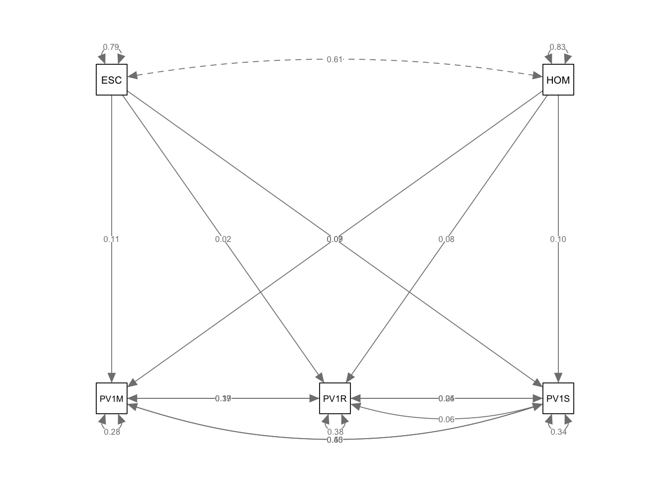
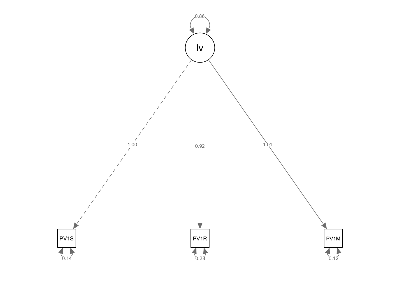
Notice the curved arrow joining the manifest variable PV1M (PV1MATH) to itself. This represents the residual variance for PV1MATH, meaning the amount of variation in PV1MATH that is not explained by the predictors PV1SCIE (science) and PV1READ (reading). The estimate of 0.219 suggests that even after accounting for science and reading scores, there is still significant unexplained variance in mathematics scores. The high z-value (69.581) and p-value (0.000) indicate that this residual variance is statistically significant.
We can make the model more complex, by adding that two of our independent variables, reading (PV1READ) and science (PV1SCIE) scores may co-vary, and vary with other independent variables. That is there is a relationship between science and reading scores. The covariance is indicated by the ~~ operator.
line 1 specify the model - recall ~ is the regression operator linking dependent and independent variable and ~~ indicates two variables covary.
2
line 2 specify that reading and science scores covary using ~~
3
line 5 create the model using the fit function
4
line 6 print the model
5
line 7 use semPath to visualise the model, specifuing that we want the coefficients printed on the lines whatLabels = "Estimate"
lavaan 0.6-20 ended normally after 23 iterations

  Estimator                                         ML
  Optimization method                           NLMINB
  Number of model parameters                        16

                                                  Used       Total
  Number of observations                         11083       12972

Model Test User Model:

  Test statistic                                    NA
  Degrees of freedom                                -4
  P-value (Unknown)                                 NA

Parameter Estimates:

  Standard errors                             Sandwich
  Information bread                           Observed
  Observed information based on                Hessian

Regressions:
                   Estimate  Std.Err  z-value  P(>|z|)
  PV1MATH ~
    PV1SCIE           0.454    0.025   18.091    0.000
    PV1READ           0.171    0.040    4.296    0.000
    ESCS              0.113    0.009   12.375    0.000
    HOMEPOS           0.071    0.009    8.126    0.000
  PV1READ ~
    PV1SCIE           0.242    0.033    7.253    0.000
    PV1MATH           0.386    0.049    7.907    0.000
 [ reached getOption("max.print") -- omitted 7 rows ]

Covariances:
                   Estimate  Std.Err  z-value  P(>|z|)
 .PV1READ ~~
   .PV1SCIE           0.065    0.014    4.786    0.000

Variances:
                   Estimate  Std.Err  z-value  P(>|z|)
   .PV1MATH           0.282    0.009   32.100    0.000
   .PV1READ           0.383    0.010   37.215    0.000
   .PV1SCIE           0.340    0.009   39.365    0.000
1.3.1 Modelling a latent variable
As introduced above, we can use SEM to model a latent variable. For example, we might assume that students have some underlying variable linked to their general intelligence. However, in the PISA data set, we have no variable that directly measures students general intelligence. We do have data on their achievement in science (PV1SCIE), mathematics (PV1MATH) and reading (PV1READ) and we might assume that as the latent variable of general achievement increases so does achievement in science, mathematics and reading.
To perform the analysis, we use the =~ operator in our model, which indicates a latent variable. This time, our model then sets out that we are interested in a lv (latent variable) which varies with science (PV1SCIE), mathematics (PV1MATH) and reading (PV1READ) scores:
model<-“lv =~ PV1SCIE + PV1READ + PV1MATH”
Then we run the model using sem in the same way as above, and plot the model using semPaths.
# For a latent variable# =~ means a latent variable1model<-"lv =~ PV1SCIE + PV1READ + PV1MATH"fit<-sem(model, data = UKdata, estimator ="MLR") summary(fit)semPaths(fit, whatLabels ="Estimate")
1
line 1 specify the latent variable using =~
lavaan 0.6-20 ended normally after 18 iterations

  Estimator                                         ML
  Optimization method                           NLMINB
  Number of model parameters                         6

  Number of observations                         12972

Model Test User Model:
                                              Standard      Scaled
  Test Statistic                                 0.000       0.000
  Degrees of freedom                                 0           0

Parameter Estimates:

  Standard errors                             Sandwich
  Information bread                           Observed
  Observed information based on                Hessian

Latent Variables:
                   Estimate  Std.Err  z-value  P(>|z|)
  lv =~
    PV1SCIE           1.000
    PV1READ           0.919    0.007  139.663    0.000
    PV1MATH           1.015    0.006  169.985    0.000

Variances:
                   Estimate  Std.Err  z-value  P(>|z|)
   .PV1SCIE           0.145    0.004   38.754    0.000
   .PV1READ           0.278    0.005   61.174    0.000
   .PV1MATH           0.119    0.003   35.189    0.000
    lv                0.855    0.012   73.665    0.000
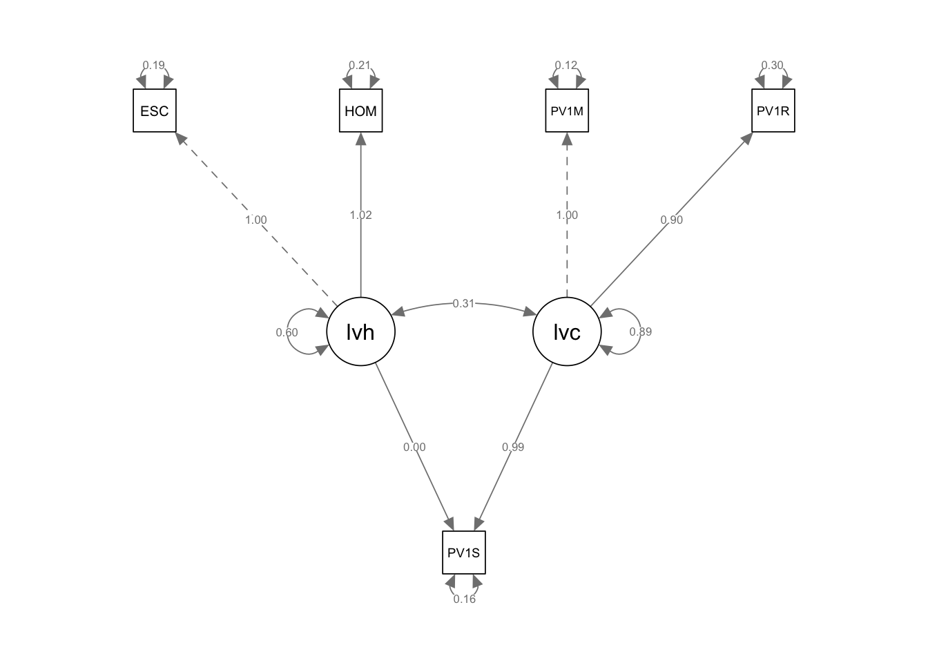
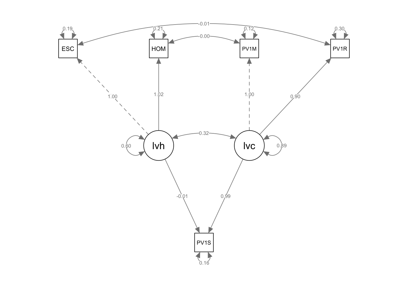
We can develop a more complex latent variable model. Let us assume that UK students’ reading scores depend on two latent variables, home environment (lvh, e.g. number of books, parental level of education etc.) and cognitive ability (lvc, e.g. as reported by science and mathematics scores). Here are the variables we will use to create the home environment latent variable:
Item name
Description
ESCS
Index of economic, social and cultural status (WLE)
HOMEPOS
Family Wealth
# Create a UK data frame with plausible valuesUKdata<-PISA_2022%>%1select(ESCS, HOMEPOS, PV1READ, PV1SCIE, PV1MATH, CNT) %>%2filter(CNT =="United Kingdom")# Scale the test scores3UKdata$PV1READ <-scale(UKdata$PV1READ)UKdata$PV1MATH <-scale(UKdata$PV1MATH)UKdata$PV1SCIE <-scale(UKdata$PV1SCIE)# Propose a model with two latent variables - one related to home (lvh), the other cognitive ability (lvc)5model<-"lvh =~ ESCS + HOMEPOS lvc =~ PV1MATH + PV1READ PV1SCIE ~ lvh + lvc"# Fit the model6fit<-sem(model, data = UKdata, estimator ="MLR")7summary(fit)semPaths(fit, whatLabels ="Estimate")
1
line 1 create the data frame for modelling, select variables of interest
2
line 4 filter for the UK
3
line 5 scale the variables to normalise all around a mean of 0 and variance 1
5
line 12 create the model using the fit function
6
line 3 print the model
7
line 4 use semPath to visualise the model, specifying that we want the coefficients printed on the lines whatLabels = "Estimate"
lavaan 0.6-20 ended normally after 29 iterations

  Estimator                                         ML
  Optimization method                           NLMINB
  Number of model parameters                        12

                                                  Used       Total
  Number of observations                         11083       12972

Model Test User Model:
                                              Standard      Scaled
  Test Statistic                                22.605      22.138
  Degrees of freedom                                 3           3
  P-value (Chi-square)                           0.000       0.000
  Scaling correction factor                                  1.021
    Yuan-Bentler correction (Mplus variant)

Parameter Estimates:

  Standard errors                             Sandwich
  Information bread                           Observed
  Observed information based on                Hessian

Latent Variables:
                   Estimate  Std.Err  z-value  P(>|z|)
  lvh =~
    ESCS              1.000
    HOMEPOS           1.023    0.019   54.796    0.000
  lvc =~
    PV1MATH           1.000
    PV1READ           0.898    0.007  127.952    0.000

Regressions:
                   Estimate  Std.Err  z-value  P(>|z|)
  PV1SCIE ~
    lvh               0.000    0.008    0.018    0.985
    lvc               0.990    0.007  134.766    0.000

Covariances:
                   Estimate  Std.Err  z-value  P(>|z|)
  lvh ~~
    lvc               0.314    0.009   35.826    0.000

Variances:
                   Estimate  Std.Err  z-value  P(>|z|)
   .ESCS              0.194    0.011   17.623    0.000
   .HOMEPOS           0.208    0.012   16.955    0.000
   .PV1MATH           0.124    0.004   32.266    0.000
   .PV1READ           0.298    0.005   58.187    0.000
   .PV1SCIE           0.158    0.004   37.002    0.000
    lvh               0.597    0.015   40.414    0.000
    lvc               0.889    0.013   67.613    0.000
Interesting features to note are a) the much higher loading of the cognitive latent variable (lvc has a loading of 0.99) than the home environment (lvh, loading 0.00); b) the roughly equal contribution of mathematics and reading scores to lvb (the cognitive ability latent variable).
Note the dotted line from the ESCS variable (truncated here to ESC) indicates that ESCS is acting as a marker variable, that is, it is fixed at 1.0, and the other variables determined relative to it. The same is true for PV1MATH for the ability latent variable.
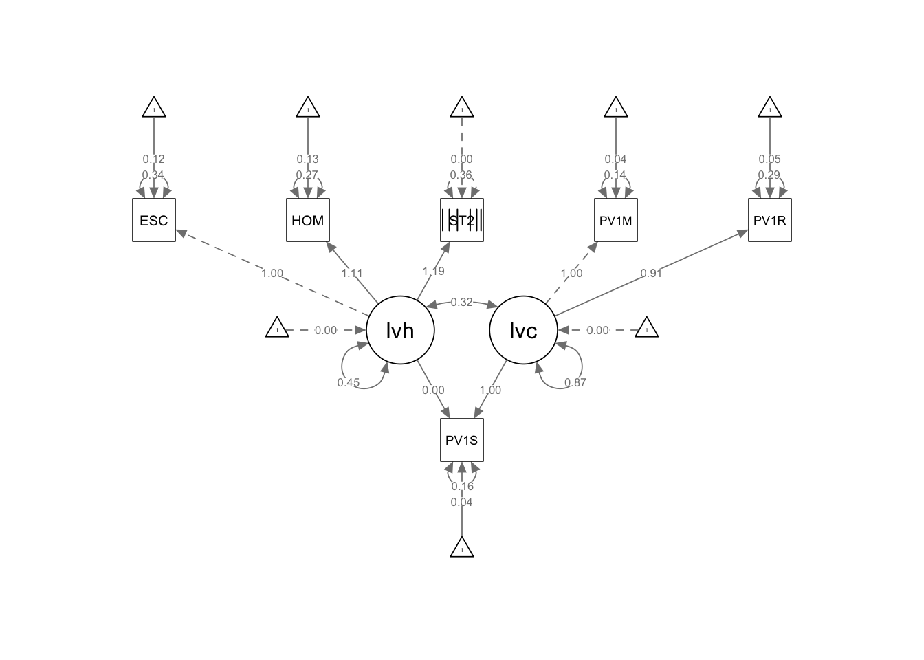
1.4 Models with categorical variables
The models above used only numeric variables, but categorical variables can also be used in SEM. For example, in the PISA data set, the variable ST255Q01JA asks “How many books are there in your home?”. We can add this item to the latent variable for the home environment (lvh). This is an ordinal variable. However, we need to indicate this variable is ordinal in three ways. First, ensure the variable is categorised as an ordinal variable (UKdata$ST255Q01JA <- as.ordered(UKdata$ST255Q01JA)). Second, in the fit function we need to label the ordinal functions. Third, we need to use a different process of estimating the model, WLSMV (Weighted Least Squares Mean and Variance-adjusted). This gives: fit <- sem(model, data = your_data, ordered = c("var2", "var3"), estimator = "WLSMV")
# Create a UK data frame with plausible valuesUKdata<-PISA_2022%>%select(ESCS, HOMEPOS, PV1READ, PV1SCIE, PV1MATH, CNT, ST255Q01JA) %>%filter(CNT =="United Kingdom") # Scale the test scoresUKdata$PV1READ <-scale(UKdata$PV1READ) UKdata$PV1MATH <-scale(UKdata$PV1MATH)UKdata$PV1SCIE <-scale(UKdata$PV1SCIE)1UKdata$ST255Q01JA <-as.ordered(UKdata$ST255Q01JA)# Propose a model with two latent variables - one related to home (lvh), the other cognitive ability (lvc)model<-"lvh =~ ESCS + HOMEPOS + ST255Q01JA lvc =~ PV1MATH + PV1READ PV1SCIE ~ lvh + lvc"# Fit the modelfit <-sem(model, UKdata, ordered =c("ST255Q01JA"), 2estimator ="WLSMV")summary(fit) semPaths(fit, whatLabels ="Estimate")
1
set the variable ST255Q01JA as an ordered variable
2
indicate that the variable ST255Q01JA is ordered and use the WLSMV estimator
Triangles have appeared which represent the threshold for the ordinal variable. A threshold in SEM refers to the value that defines the boundary between categories of an ordinal variable - in this case the number of books in the home. The variable ST255Q01JA in your data represents a set of ordered categories about the number of books. For example: “There are no books” ; 1-10 books.” “11-25 books.” … (and so on).
The bars on the squares are visual markers that indicate which variables are being treated as ordinal variables in the model. In your case, you’ve specified ST255Q01JA as an ordinal variable by using the as.ordered() function. The bars are a way of indicating that ST255Q01JA is not a continuous variable but an ordinal one, which reflects a ranked or ordered scale.
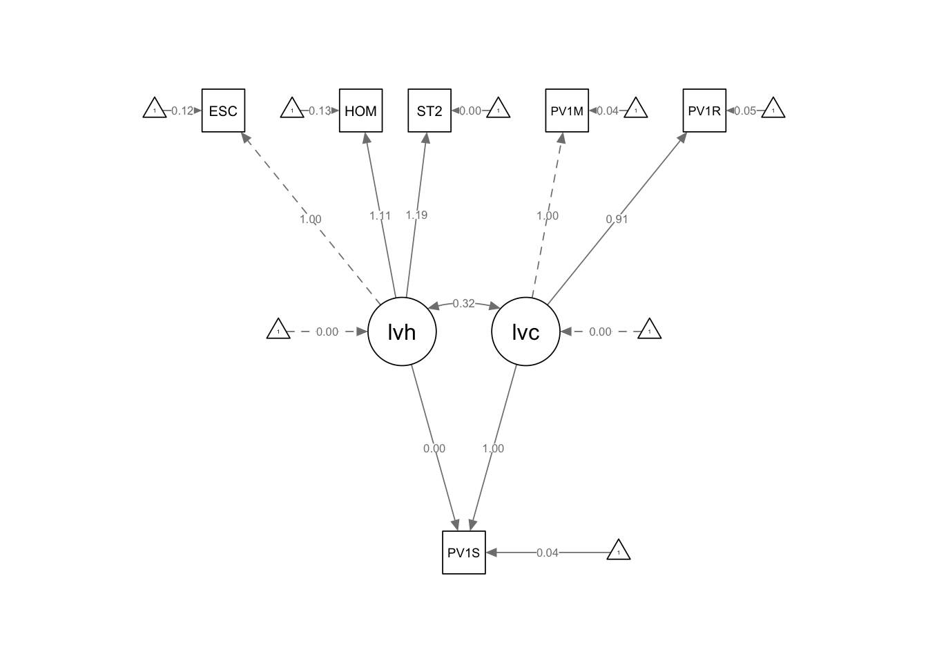
Tip
If adding an ordinal variable, with the addition of triangles to the plot, makes your path diagram too crowded, you can turn off estimates for thresholds and residual variances as follows:
If you want to link an ordinal variable directly to an outcome variable, for example, if you want to link books directly to reading, doing it through a latent variable allows lavaan to estimate the thresholds for the ordinal variable.
To fit a categorical variable like gender, you can use the as.factor function to convert the variable to a factor and then use the fit <- sem(model, UKdata, estimator = "MLR") function to estimate the model. MLR is the default estimator for categorical variables. MLR stands for Maximum Likelihood Robust. It is an estimator used in structural equation modeling (SEM), particularly when dealing with non-normal data or small sample sizes. See the example below using gender:
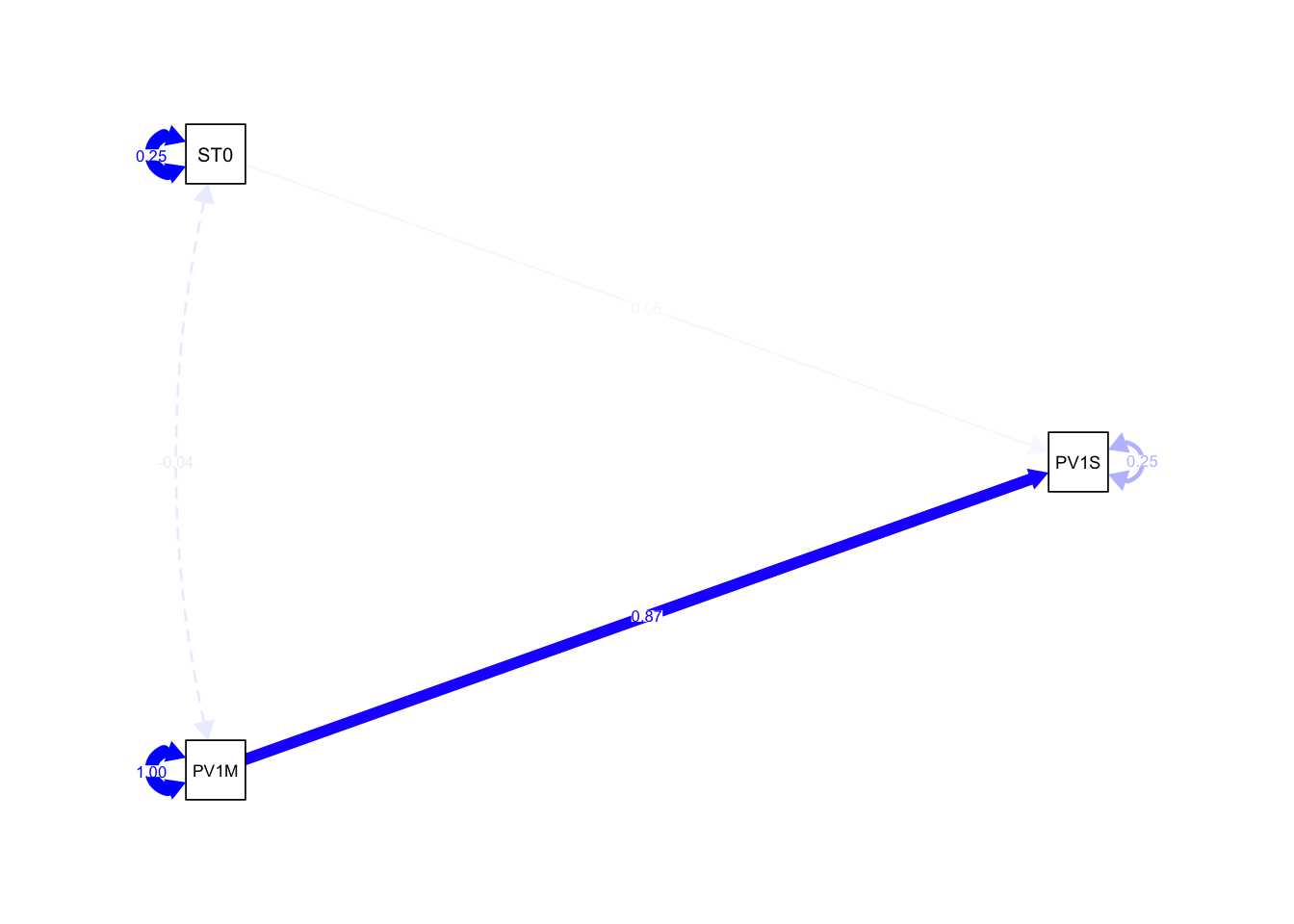
# Create a data frame with the required base variablesUKdata<-PISA_2022 %>%select(CNT, PV1SCIE, PV1MATH, ST004D01T) %>%filter(CNT =="United Kingdom") %>%na.omit() # Remove the NAs to create a two level variable.# set ST004D01T to a factorUKdata$ST004D01T <-factor(UKdata$ST004D01T, levels =c("Male", "Female"))# Scale the numeric variablesUKdata <- UKdata %>%mutate(PV1SCIE =scale(PV1SCIE),PV1MATH =scale(PV1MATH))# Create the modelmodel <-"PV1SCIE ~ PV1MATH + ST004D01T"fit <-sem(model, data = UKdata, estimator ="MLR")summary(fit)
lavaan 0.6-20 ended normally after 1 iteration
Estimator ML
Optimization method NLMINB
Number of model parameters 3
Number of observations 12972
Model Test User Model:
Standard Scaled
Test Statistic 0.000 0.000
Degrees of freedom 0 0
Parameter Estimates:
Standard errors Sandwich
Information bread Observed
Observed information based on Hessian
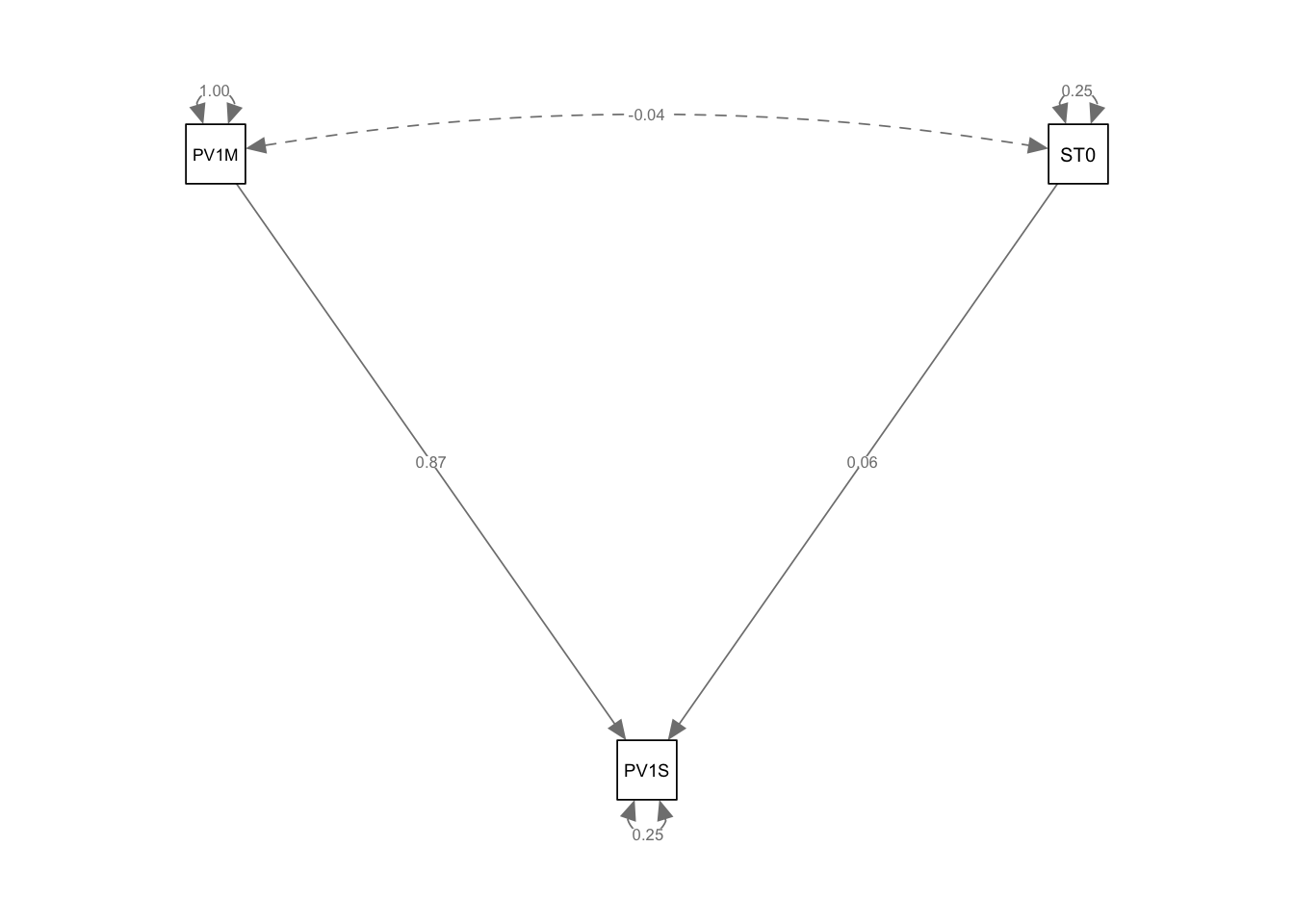
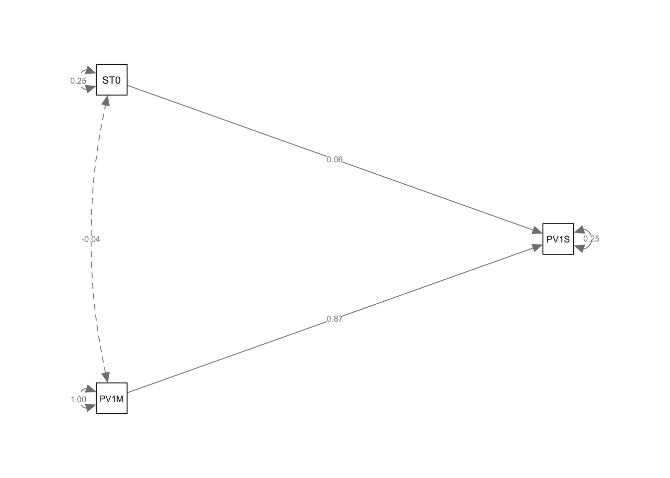
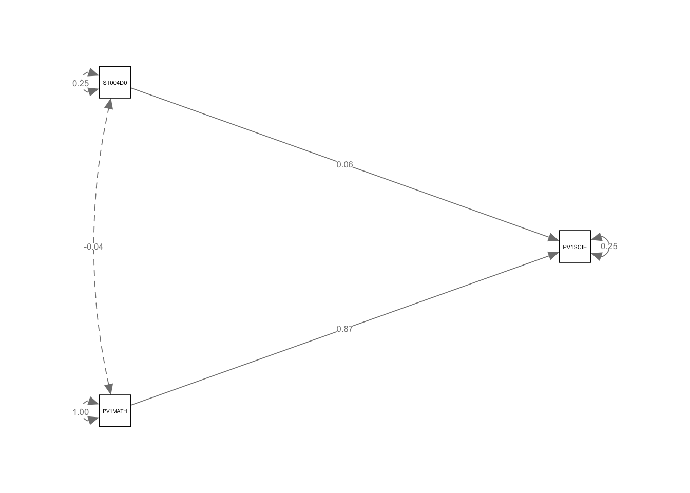
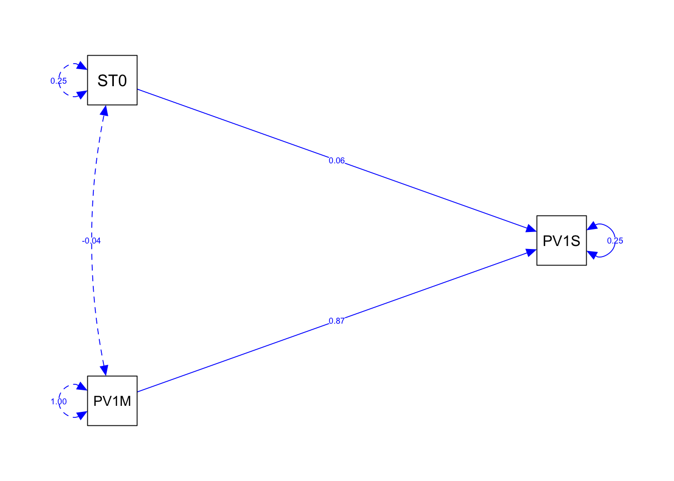
Regressions:
Estimate Std.Err z-value P(>|z|)
PV1SCIE ~
PV1MATH 0.870 0.004 196.331 0.000
ST004D01T 0.056 0.009 6.457 0.000
Variances:
Estimate Std.Err z-value P(>|z|)
.PV1SCIE 0.246 0.003 73.035 0.000
semPaths(fit, whatLabels ="Estimate")
Tip
If you have both categorical and ordinal variables, it’s best to use WLSMV because it can appropriately handle both ordinal variables (using thresholds) and categorical variables (using multinomial logistic regression), while also providing correct standard errors.
1.5 Labelling paths to calculate indirect effects
In SEM, indirect effects occur when the effect of one variable on another is mediated through one or more intervening variables. To calculate indirect effects in lavaan, you need to label the paths in your model using the label argument. This allows you to specify which paths you want to include in the calculation of indirect effects.
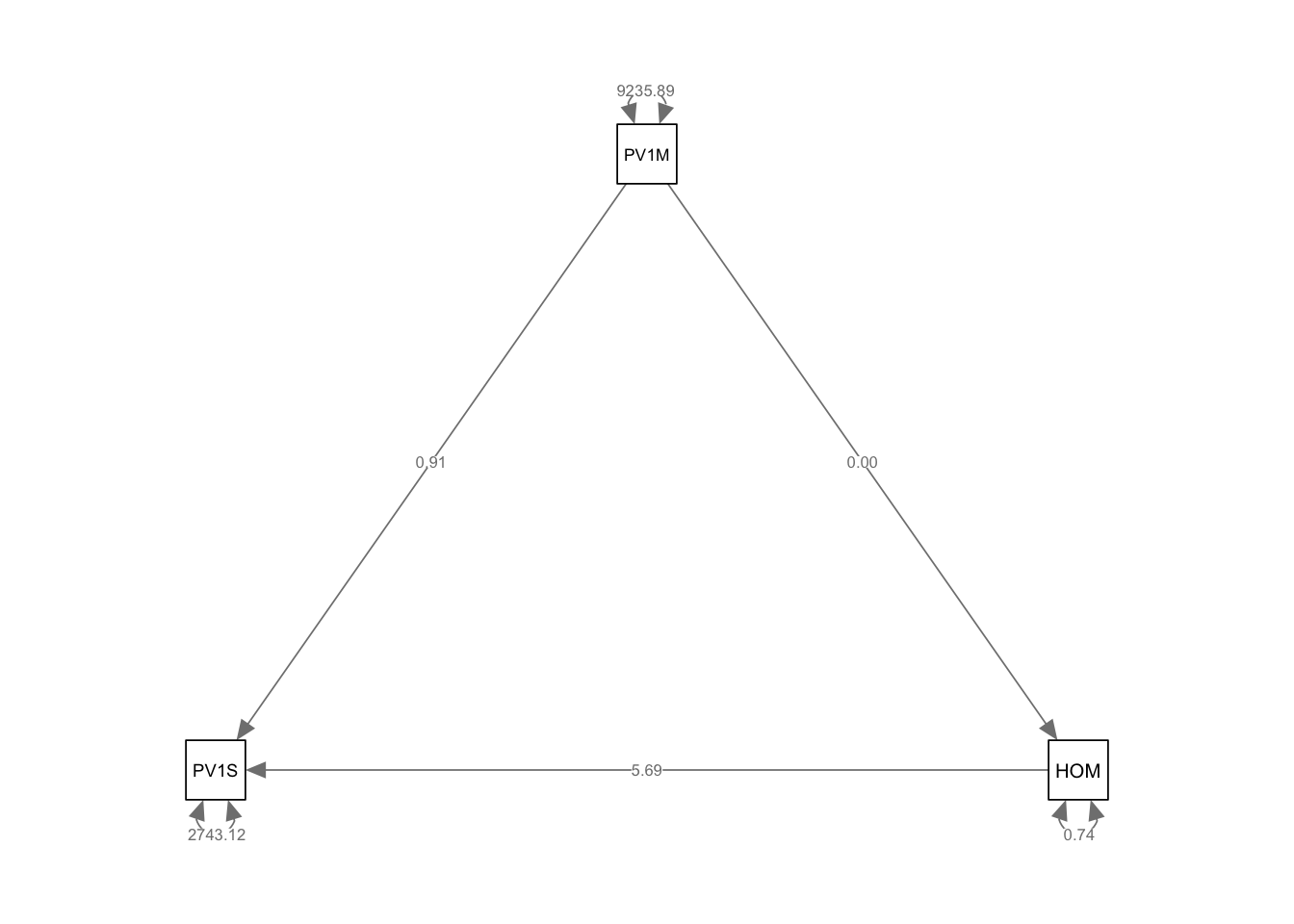
For example, consider a model where variable PV1MATH (math score) affects variable PV1SICE (science score) through a mediator variable HOMEPOS (wealth). We add coefficients to the paths using labels a, b and c, and then define the indirect effect as the product of the paths a and c. Note we use the operator := to define the indirect effect.
# Create a data frame with the required variablesUKdata <- PISA_2022 %>%select(CNT, HOMEPOS, PV1MATH, PV1SCIE) %>%filter(CNT =="United Kingdom") model <-" PV1SCIE ~ a*PV1MATH + b*HOMEPOS HOMEPOS ~ c*PV1MATH # Indirect effect indirect_effect := a * c"fit <-sem(model, data = UKdata, estimator ="MLR")summary(fit, standardized =TRUE, fit.measures =TRUE)
lavaan 0.6-20 ended normally after 1 iteration

  Estimator                                         ML
  Optimization method                           NLMINB
  Number of model parameters                         5

                                                  Used       Total
  Number of observations                         11487       12972

Model Test User Model:
                                              Standard      Scaled
  Test Statistic                                 0.000       0.000
  Degrees of freedom                                 0           0

Model Test Baseline Model:

  Test statistic                             17314.368   14282.056
  Degrees of freedom                                 3           3
  P-value                                        0.000       0.000
  Scaling correction factor                                  1.212

User Model versus Baseline Model:

  Comparative Fit Index (CFI)                    1.000       1.000
  Tucker-Lewis Index (TLI)                       1.000       1.000

  Robust Comparative Fit Index (CFI)                            NA
  Robust Tucker-Lewis Index (TLI)                               NA

Loglikelihood and Information Criteria:

  Loglikelihood user model (H0)             -76323.012  -76323.012
  Loglikelihood unrestricted model (H1)     -76323.012  -76323.012

  Akaike (AIC)                              152656.024  152656.024
  Bayesian (BIC)                            152692.769  152692.769
  Sample-size adjusted Bayesian (SABIC)     152676.880  152676.880

Root Mean Square Error of Approximation:

  RMSEA                                          0.000          NA
  90 Percent confidence interval - lower         0.000          NA
  90 Percent confidence interval - upper         0.000          NA
  P-value H_0: RMSEA <= 0.050                       NA          NA
  P-value H_0: RMSEA >= 0.080                       NA          NA

  Robust RMSEA                                               0.000
  90 Percent confidence interval - lower                     0.000
  90 Percent confidence interval - upper                     0.000
  P-value H_0: Robust RMSEA <= 0.050                            NA
  P-value H_0: Robust RMSEA >= 0.080                            NA

Standardized Root Mean Square Residual:

  SRMR                                           0.000       0.000

Parameter Estimates:

  Standard errors                             Sandwich
  Information bread                           Observed
  Observed information based on                Hessian

Regressions:
                   Estimate  Std.Err  z-value  P(>|z|)   Std.lv  Std.all
  PV1SCIE ~
    PV1MATH    (a)    0.914    0.006  165.914    0.000    0.914    0.845
    HOMEPOS    (b)    5.687    0.585    9.727    0.000    5.687    0.050
  HOMEPOS ~
    PV1MATH    (c)    0.003    0.000   39.705    0.000    0.003    0.355

Variances:
                   Estimate  Std.Err  z-value  P(>|z|)   Std.lv  Std.all
   .PV1SCIE        2743.115   38.628   71.013    0.000 2743.115    0.254
   .HOMEPOS           0.738    0.013   55.888    0.000    0.738    0.874

Defined Parameters:
                   Estimate  Std.Err  z-value  P(>|z|)   Std.lv  Std.all
    indirect_effct    0.003    0.000   38.391    0.000    0.003    0.300
semPaths(fit, whatLabels ="Estimate")
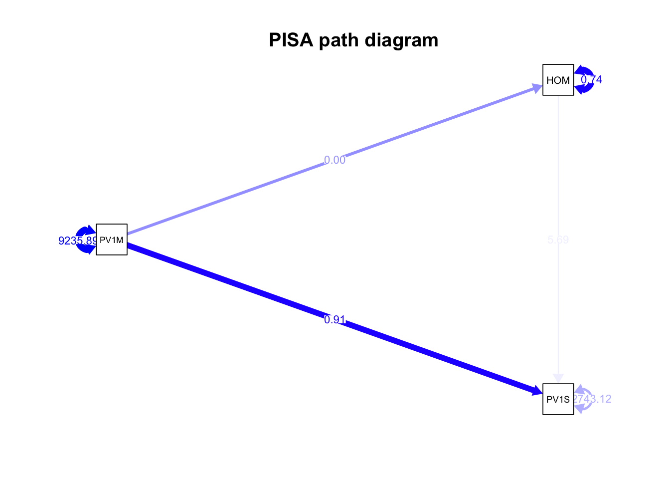
In this example, the paths from PV1MATH to PV1SCIE and from PV1MATH to HOMEPOS are labeled as a and c, respectively. The indirect effect of PV1MATH on PV1SCIE through HOMEPOS is then calculated as the product of these two paths (indirect_effect := a * c). Here we find the coefficient for the indirect effect is only 0.003, indicating a very small indirect effect of mathematics score on science score through wealth.
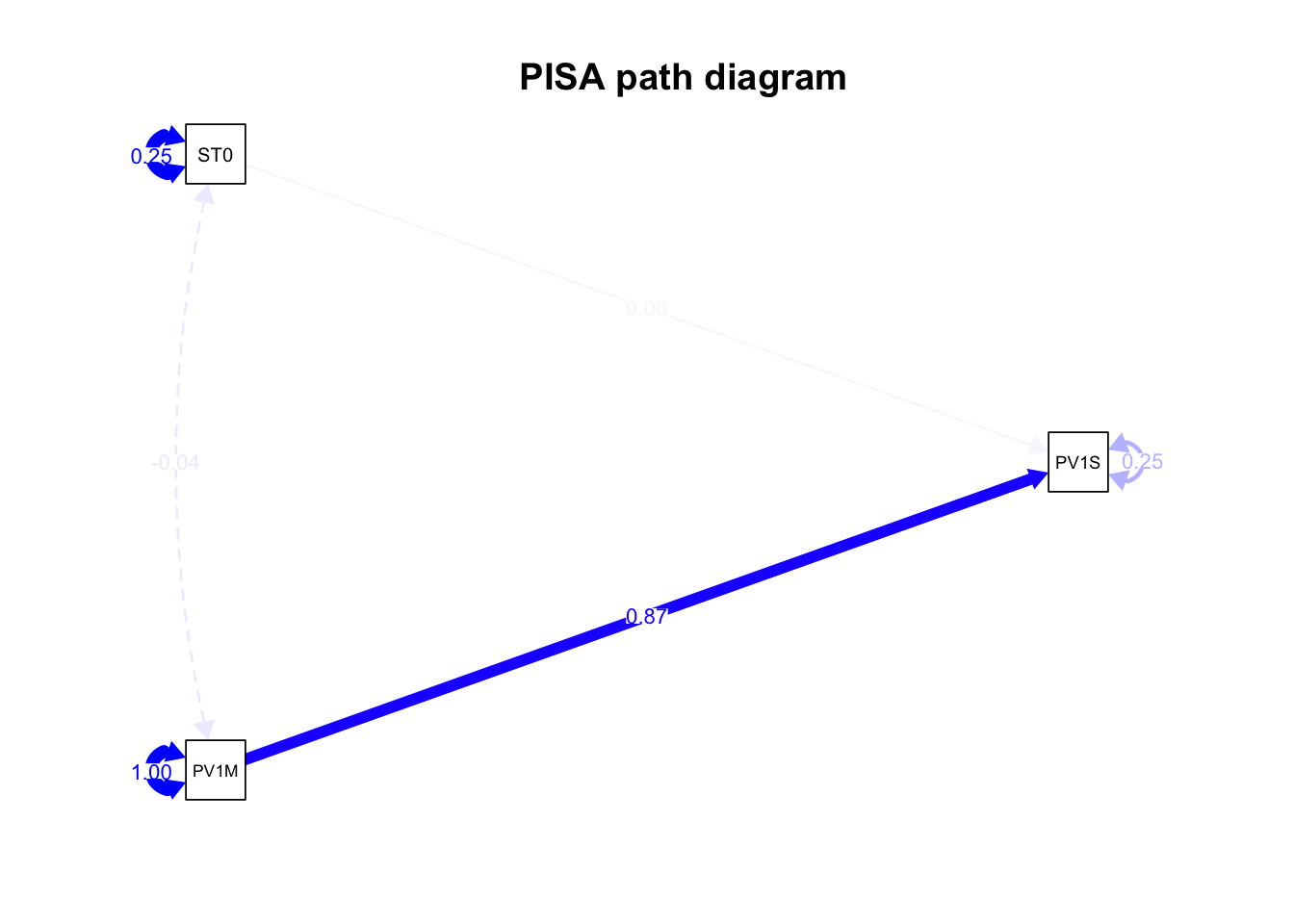
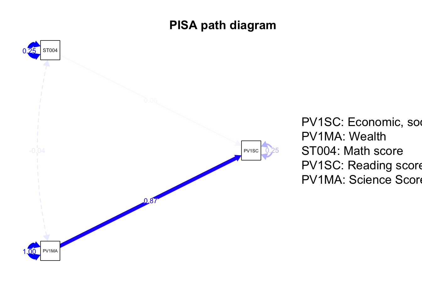
To give longer node names (nodeNames=nodenames), and you can increase the abbreviation of labels to a set number of characters in the nodes using nCharNodes = 3. node.label.cex sets the size of the node label text:
nodenames<-c("Economic, social and cultural status","Wealth", "Math score", "Reading score", "Science Score")semPaths(fit, whatLabels ="Estimate", rotation=2, edge.color ="blue", sizeMan =5, "std", edge.label.cex =0.8, nodeNames = nodenames,nCharNodes =5)title("PISA path diagram")
Tip
You can find more information on formatting path diagrams using semPaths on semptools and on the Comprehensive R Archive network (CRAN) documentation for the package.
1.7 Estimating model fit
After running a SEM, it is important to determine how well the model fits the data. There are a number of different measures of model fit, no one measure provides a definitive measure of the fit - it is best practice to consider a number of different indicators and come to a holistic judgement. Measures include:
The Chi-Square Test of Model Fit Assume the null hypothesis that the model fits the data well. A non-significant p-value indicates good fit. However, this test is sensitive to sample size, and with large samples, even minor deviations may be significant: ‘[Chi-square] is sensitive to sample size because as sample size increases (generally above 200), the χ2 has a tendency to indicate a significant probability level’ (Schumacker and Lomax 2004, 92).
Comparative Fit Index (CFI) and Tucker-Lewis Index (TLI) Values closer to 1 indicate better fit. Common thresholds for the two indicies are Acceptable fit: > 0.90 Good fit: > 0.95 (Kline 2023, 204; McDonald and Ho 2002)
Root Mean Square Error of Approximation (RMSEA) A measure of approximate fit in the population. Common thresholds: Good fit: < 0.06 Acceptable fit: < 0.08 Look at the 90% confidence interval for RMSEA as well.
To get estimates of model fit, when you run the summary command, include: summary(fit, fit.measures = TRUE)
For example:
# Create a UK data frame with plausible valuesUKdata<-PISA_2022 %>%1select(CNT, ESCS, HOMEPOS, PV1READ, PV1SCIE, PV1MATH)%>%2filter(CNT =="United Kingdom")# Scale the test scores3UKdata$PV1READ <-scale(UKdata$PV1READ)UKdata$PV1MATH <-scale(UKdata$PV1MATH)UKdata$PV1SCIE <-scale(UKdata$PV1SCIE)# Propose a model with two latent variables - one related to home (lvh), the other cognitive ability (lvc)4model<-"lvh =~ ESCS + HOMEPOS lvc =~ PV1MATH + PV1READ PV1SCIE ~ lvh + lvc"# Fit the model5fit<-sem(model, data = UKdata)6summary(fit, fit.measures =TRUE)7semPaths(fit, whatLabels ="Estimate")
1
line 1 create the data frame for modelling, select variables of interest
2
line 4 filter for the UK
3
line 8 scale the variables to normalise all around a mean of 0 and variance 1
4
line 11 specify the model - note that two latent variables are proposed (lvh, lvc) - these are specified using the =~ operator
5
line 12 create the model using the fit function
6
line 3 print the model - fit.measures = TRUE reports the fit parameters
7
line 4 use semPath to visualise the model, specifying that we want the coefficients printed on the lines whatLabels = "Estimate"
lavaan 0.6-20 ended normally after 29 iterations

  Estimator                                         ML
  Optimization method                           NLMINB
  Number of model parameters                        12

                                                  Used       Total
  Number of observations                         11083       12972

Model Test User Model:

  Test statistic                                22.605
  Degrees of freedom                                 3
  P-value (Chi-square)                           0.000

Model Test Baseline Model:

  Test statistic                             37896.675
  Degrees of freedom                                10
  P-value                                        0.000

User Model versus Baseline Model:

  Comparative Fit Index (CFI)                    0.999
  Tucker-Lewis Index (TLI)                       0.998

Loglikelihood and Information Criteria:

  Loglikelihood user model (H0)             -57695.609
  Loglikelihood unrestricted model (H1)     -57684.307

  Akaike (AIC)                              115415.218
  Bayesian (BIC)                            115502.976
  Sample-size adjusted Bayesian (SABIC)     115464.842

Root Mean Square Error of Approximation:

  RMSEA                                          0.024
  90 Percent confidence interval - lower         0.016
  90 Percent confidence interval - upper         0.034
  P-value H_0: RMSEA <= 0.050                    1.000
  P-value H_0: RMSEA >= 0.080                    0.000

Standardized Root Mean Square Residual:

  SRMR                                           0.004

Parameter Estimates:

  Standard errors                             Standard
  Information                                 Expected
  Information saturated (h1) model          Structured

Latent Variables:
                   Estimate  Std.Err  z-value  P(>|z|)
  lvh =~
    ESCS              1.000
    HOMEPOS           1.023    0.019   54.286    0.000
  lvc =~
    PV1MATH           1.000
    PV1READ           0.898    0.007  130.208    0.000

Regressions:
                   Estimate  Std.Err  z-value  P(>|z|)
  PV1SCIE ~
    lvh               0.000    0.008    0.019    0.985
    lvc               0.990    0.007  137.089    0.000

Covariances:
                   Estimate  Std.Err  z-value  P(>|z|)
  lvh ~~
    lvc               0.314    0.009   35.365    0.000

Variances:
                   Estimate  Std.Err  z-value  P(>|z|)
   .ESCS              0.194    0.010   18.471    0.000
   .HOMEPOS           0.208    0.011   18.898    0.000
   .PV1MATH           0.124    0.004   33.351    0.000
   .PV1READ           0.298    0.005   61.818    0.000
   .PV1SCIE           0.158    0.004   40.379    0.000
    lvh               0.597    0.014   41.261    0.000
    lvc               0.889    0.014   63.886    0.000
Going through the fit measures of that model:
P-value (Chi-square) 0.000
The p-value is less than 0.05 suggesting a poor fit
Comparative Fit Index (CFI) 0.999 Tucker-Lewis Index (TLI) 0.9998
The CFI and TLI are over 0.95 suggesting a good fit
The RMS error term is 0.024 with the 90% confidence interval between 0.016 and 0.034 An RMSEA of 0.024 suggests good fit, as it is under common thresholds for acceptable fit: Good fit: < 0.06; Acceptable fit: 0.06–0.08 and Poor fit: > 0.08.
As is commonly the case, the model indicators make different suggestions of the goodness of the model’s fit. Overall this seems like not the best fitting model.
1.7.1 Local fit
Alongside checking the overall fit of the model, it is also important to check the local fit of the model. Local fit looks at how well individual parts of the model fit the data. One way to look at local fit is to examine the standardised residuals. Standardised residuals are the differences between the observed and predicted values, scaled by the standard deviation. Large residuals indicate areas where the model does not fit well.
The table output suggest ways to improve the model to improve the fit. One should be cautious about making changes to a model based purely on such modification indices. The model should fit theory. The lhs and rhs columns refer to the left hand side and right hand side of the equation. The ops column refers to the operator, this suggests the type of relationship that might be added to improve the model:
~~ (Covariance or Correlation) - you might add: ‘ESCS ~~ PV1READ’ to the model
=~ (Latent Variable Measurement Relationship) - suggests adding a new aspect to the home latent variable in the model: lvh =~ PV1READ
Note, that the suggestions here are purely numeric. It does not take into account the theoretical coherence of the model. For example, adding reading scores to the home environment latent variable (lvh =~ PV1READ) does not make much sense.
The suggestions to improve are ranked by the mi improvement. mi is a measure of how much the models chi-square value would decrease if you added the additional term. For example, adding ESCS ~~ PV1READ would bring the chi-square value down by 18.099.
The epc is the Expected Parameter Change - the expected value of the new term (covariance, or factor loading). For example, looking at the epc term for ESCS ~~ PV1READ - if this term were added to the model, that relationship would be expected to have a covariance of -0.014.
We can then add the suggested terms and compare model fit, adding the top two suggestions: ESCS ~~ PV1READ (a covariance between social class and reading score) and ESCS ~~ PV1MATH (a covariance between class and mathematics scores) . It is important to check those additions cohere with theory. A link between class and reading and mathematics score seems plausible from knowledge of the link between class and achievement in the literature.
# Propose a modified model model2<-"lvh =~ ESCS + HOMEPOS lvc =~ PV1MATH + PV1READ PV1SCIE ~ lvh + lvc ESCS ~~ PV1READ HOMEPOS ~~ PV1MATH"# Fit the modelfit<-sem(model2, data = UKdata) summary(fit, , fit.measures =TRUE)
lavaan 0.6-20 ended normally after 34 iterations

  Estimator                                         ML
  Optimization method                           NLMINB
  Number of model parameters                        14

                                                  Used       Total
  Number of observations                         11083       12972

Model Test User Model:

  Test statistic                                 2.529
  Degrees of freedom                                 1
  P-value (Chi-square)                           0.112

Model Test Baseline Model:

  Test statistic                             37896.675
  Degrees of freedom                                10
  P-value                                        0.000

User Model versus Baseline Model:

  Comparative Fit Index (CFI)                    1.000
  Tucker-Lewis Index (TLI)                       1.000

Loglikelihood and Information Criteria:

  Loglikelihood user model (H0)             -57685.571
  Loglikelihood unrestricted model (H1)     -57684.307

  Akaike (AIC)                              115399.142
  Bayesian (BIC)                            115501.527
  Sample-size adjusted Bayesian (SABIC)     115457.036

Root Mean Square Error of Approximation:

  RMSEA                                          0.012
  90 Percent confidence interval - lower         0.000
  90 Percent confidence interval - upper         0.031
  P-value H_0: RMSEA <= 0.050                    1.000
  P-value H_0: RMSEA >= 0.080                    0.000

Standardized Root Mean Square Residual:

  SRMR                                           0.002

Parameter Estimates:

  Standard errors                             Standard
  Information                                 Expected
  Information saturated (h1) model          Structured

Latent Variables:
                   Estimate  Std.Err  z-value  P(>|z|)
  lvh =~
    ESCS              1.000
    HOMEPOS           1.022    0.020   52.298    0.000
  lvc =~
    PV1MATH           1.000
    PV1READ           0.898    0.007  130.237    0.000

Regressions:
                   Estimate  Std.Err  z-value  P(>|z|)
  PV1SCIE ~
    lvh              -0.007    0.008   -0.833    0.405
    lvc               0.993    0.007  135.416    0.000

Covariances:
                   Estimate  Std.Err  z-value  P(>|z|)
 .ESCS ~~
   .PV1READ          -0.013    0.003   -3.703    0.000
 .HOMEPOS ~~
   .PV1MATH          -0.004    0.003   -1.385    0.166
  lvh ~~
    lvc               0.318    0.009   35.568    0.000

Variances:
                   Estimate  Std.Err  z-value  P(>|z|)
   .ESCS              0.193    0.011   17.655    0.000
   .HOMEPOS           0.209    0.011   18.319    0.000
   .PV1MATH           0.125    0.004   33.448    0.000
   .PV1READ           0.298    0.005   61.787    0.000
   .PV1SCIE           0.158    0.004   40.228    0.000
    lvh               0.598    0.015   40.357    0.000
    lvc               0.889    0.014   63.864    0.000
semPaths(fit, whatLabels ="Estimate")
If we compare the model fit indices in the improved model to the original:
Fit Measure
Model 1
Model 2
Improvement?
Comments on Change
Chi-Square
2.529 (df = 1, p = 0.112)
2.529 (df = 1, p = 0.112)
No Change
Both models have identical chi-square values, indicating no improvement.
CFI (Comparative Fit Index)
1.000
1.000
No Change
No change in CFI, both models show perfect fit.
TLI (Tucker-Lewis Index)
1.000
1.000
No Change
TLI remains the same for both models, indicating no difference in model fit.
RMSEA
0.012
0.012
No Change
RMSEA is the same in both models, suggesting that fit in terms of RMSEA did not change.
There is no difference in terms of model fit indicators between Model 1 and Model 2. Both models show identical values for Chi-Square, CFI, TLI, RMSEA, SRMR, and other fit indices, indicating that the models are performing equivalently. As the first model fit was relatively high, there was limited scope for improvement here.
1.8.1 Reporting the model
Once you have finalised your model, you will want to report various aspects of your SEM. Typically you will be interested in the factor loadings (the standardised coefficients representing the paths between variables). The loadings are displayed on your path diagram but you can produce an output of the loadings separately. For example for model2 above which attempts to model science scores with a latent home and cognitive item, you can extract the factor loadings using the standardizedsolution function.
# Report the modelmodel2<-"lvh =~ ESCS + HOMEPOS lvc =~ PV1MATH + PV1READ PV1SCIE ~ lvh + lvc ESCS ~~ PV1READ HOMEPOS ~~ PV1MATH"# Fit the modelfit<-sem(model2, data = UKdata) # Extract loadingsstandardizedsolution(fit)
The output table gives you a list of the factor loadings between pairs of variables. For example, the first pair is the latent variable for the home environment (lvh) and social class (ESCS). The loading estimate is given in the est.std column - 0.870 in this case. The columns ci.lower and ci.upper give the 95% confidence interval for the loading.The pvalue column returns the p-value for the loading. There is no well defined cut off in the literature, but if you have variables that have low loadings you may wish to reconsider their inclusion in the model.
Tip
There is disagreement in the literature as concerns the cut off for low factor loading. For example Hulland (1999) suggests adopting the value commonly used in factor analysis, < 0.4. By contrast, Fornell and Larcker (1981) recommend 0.7 and Chin (1998) prefers 0.707. Decisions will be field dependent so it is worth reading papers in your field to get a sense of the conventions in your discipline.
Another useful measure are the R2 values for each item in the model. Each item is treated as a dependent variable and an R2 value (the proportion of variance it explains) can be calculated using the parameterEstimates function. We then filter for the operator related to R2 and select the relevant columns to make the data easier to read. An arrange in descending order can also be useful.
The estimates here should be thought of as the percentage of variance of that item that is explained by the latent variable it is associated with.
# Extract R^2 values for the modelparameterEstimates(fit, rsquare =TRUE) %>%filter(op =="r2") %>%select(Item=rhs, R2 = est) %>%arrange(desc(R2))
For example, ESCS in the model is associated with lvh, the home environment latent variable. Therefore the R2 value here indicates that 75.6% of the variance in ESCS is explained by lvh.
1.9 Seminar activities
1.9.1 Task 1 - create a model of science score
Consider the mathematics score in the PISA data (PV1SCIE). On a piece of paper, draw out a path diagram of the variables that might influence science score. Try and estimate the relative strength of the effect of those variables on mathematics score. You might consider variables such as IQ and teacher_quality.
1.9.2 Task 2 - simple models of achievement
Try to create an SEM for science score in the UK. Let us assume that the variables theory suggest you include in your model are ability at mathematics and reading (PV1MATH and PV1READ) and wealth (HOMEPOS). Build a simple model in which those three variables have a direct relationship to science score, but don’t influence each other. Describe what your model suggests about the relationship between the variables.
Answer
# Create a data frame for UK science scores, with the variables we need# For the model: Math, science, reading and wealth (HOMEPOS)UK_Sci_data <- PISA_2022 %>%select(CNT, HOMEPOS, PV1READ, PV1SCIE, PV1MATH) %>%filter(CNT =="United Kingdom")# Scale the the test scores so they are similar to the already scaled# HOMEPOS score (i.e. have a mean of 0 and a sd of 1)UK_Sci_data <- UK_Sci_data %>%mutate(PV1MATH =scale(PV1MATH),PV1SCIE =scale(PV1SCIE),PV1READ =scale(PV1READ))model<-"PV1SCIE ~ HOMEPOS + PV1MATH + PV1READ"fit<-sem(model, data = UK_Sci_data, estimator ="MLR")summary(fit)semPaths(fit, whatLabels ="Estimate")# Science is most influenced by mathematics scores in this model (factor loading = 0.66), following# by a smaller impact of reading (0.25). When the two academic scores are taken into account# wealth (HOMEPOS) doesn't exert a large influence on science scores. The relatively high covariance# between reading and mathematics scores (0.81) suggests this is not a great model. The residual term # variance of 23.9% suggests that a significant portion of the variance in science scores is unexplained by the model.
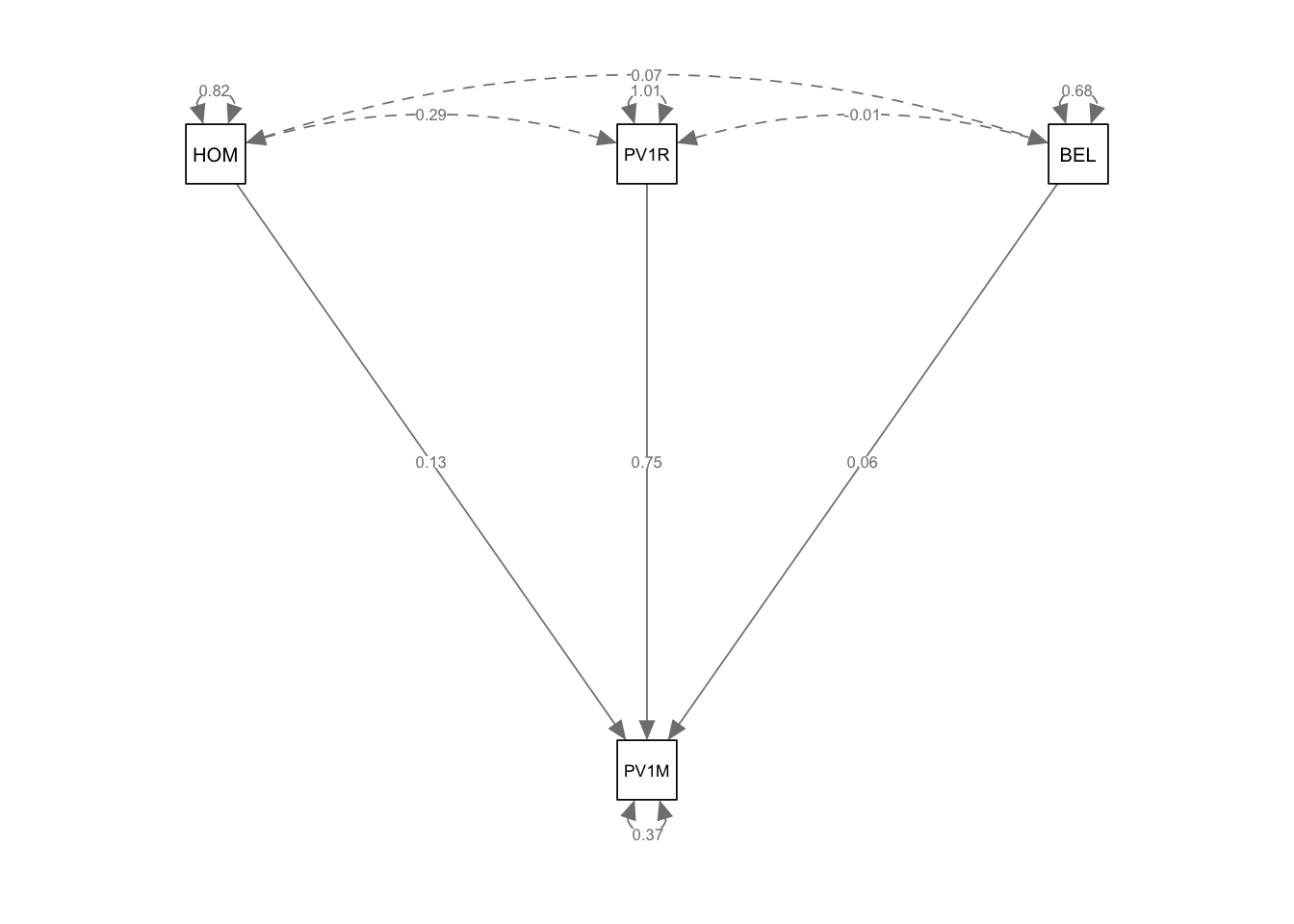
Try to create an SEM for mathematics score in the UK. Let us assume that the variables theory suggest you include in your model are ability at reading (PV1READ) and wealth (HOMEPOS) and sense of belonging (BELONG). Build a simple model in which those three variables have a direct relationship to mathematics score, but don’t influence each other. Describe what your model suggests about the relationship between the variables.
Answer
# Create a data frame for UK math scores, with the variables we need# For the model: Math, reading, wealth (HOMEPOS) and class (BELONG)UK_math_data <- PISA_2022 %>%select(CNT, HOMEPOS, PV1READ, PV1MATH, BELONG) %>%filter(CNT =="United Kingdom")# Scale the the test scores so they are similar to the already scaled# HOMEPOS score (i.e. have a mean of 0 and a sd of 1)UK_math_data <- UK_math_data %>%mutate(PV1MATH =scale(PV1MATH),PV1READ =scale(PV1READ))model<-"PV1MATH ~ HOMEPOS + PV1READ + BELONG"fit<-sem(model, data = UK_math_data)summary(fit)semPaths(fit, whatLabels ="Estimate")# This regression shows a positive and statistically significant relationship between HOMEPOS (wealth) and PV1MATH (Math scores). The relationship is statistically signifcant (p<0.05). or each unit increase in HOMEPOS, PV1MATH increases by 0.126 units. This shows a very strong (0.753) and significant relationship between PV1READ (Reading scores) and PV1MATH (Math scores). The weakest relationship is between BELONG and PV1MATH (0.055). The residual variance in PV1MATH (math scores), which is the part of the math score variance not explained by the predictors HOMEPOS, PV1READ, and BELONG. The estimate of 0.372 suggests that a significant amount of variance in PV1MATH remains unexplained, even after accounting for the predictors.
Create your own SEM using any continuous variables in some country (e.g, PV1READ, HOMEPOS, BELONG etc.). Describe what your model suggests about the relationship between the variables.
1.9.3 Task 3 - a model with a latent variable
Performance in science (PV1READ) might be thought to depend on two latent variables. Cognitive ability (you might label this cog) - which loads on PV1MATH and PV1SCIE and the home environment (home) which loads on wealth (HOMEPOS) and social class (ESCS)
Build an SEM model of reading achievement in the UK with these two latent variables and comment on what the model shows you.
Answer
# Create data setUKdata <- PISA_2022 %>%select(CNT, PV1SCIE, PV1MATH, PV1READ, HOMEPOS, ESCS) %>%filter(CNT =="United Kingdom") # Set up the model withmodel<-"PV1MATH ~ cog + home cog =~ PV1READ + PV1SCIE home =~ HOMEPOS + ESCS "fit <-sem(model, data = UKdata, estimator ="MLR")summary(fit)semPaths(fit, whatLabels ="Estimate")
1.9.4 Task 4 - a more complex latent variable
Performance in science (PV1MATH) might be thought to depend on a number of latent variables. For example, a latent variable related to cognitive ability (you might label this cog) to school variables (sch) and to the home environment (home).
Build an SEM model of science achievement in Hong Kong (China) (chosen as it has the least missing data) with these three latent variables and comment on what the model shows you.
Variables that might be of interest include:
Item name
Description
HOMEPOS
Family Wealth
ESCS
Index of economic, social and cultural status
BELONG
Sense of belonging
PARINVOL
Parental involvement
DISCLIM
Disciplinary climate in mathematics (WLE)”
BULLIED
Bullied at school
PV1SCIE
Science score
PV1MATH
Mathematics score
PV1READ
Reading score
Answer
# Create data setHKdata <- PISA_2022 %>%select(CNT, PV1SCIE, PV1MATH, PV1READ, HOMEPOS, ESCS, BELONG, PARINVOL, DISCLIM, BULLIED) %>%filter(CNT =="Hong Kong (China)") # Set up the model with# Cogntive latent variable (cog) - based on academic scores PV1READ and PV1SCIE# Home latent variable (home) - based on HOMEPOS (wealth), ESCS (social class), PARINVOL (parental involvement)# School latent variable (sch) - based on DISCLIM (discipline in maths), BULLIED (level of bullying), BELONG (sense of belonging)model<-"PV1MATH ~ cog + home + sch cog =~ PV1READ + PV1SCIE home =~ HOMEPOS + ESCS + PARINVOL sch =~ DISCLIM + BULLIED + BELONG PV1SCIE ~ PV1MATH"fit <-sem(model, data = HKdata, estimator ="MLR")summary(fit)semPaths(fit, whatLabels ="Estimate")
1.9.5 Task 5 - models with categorical variables
Create a model of mathematics scores in the UK, using the predictors gender (ST004D01T), reading score (PV1READ), wealth (HOMEPOS), and social class (ESCS).
Hint: remember to turn gender into a factor variable and use estimator = "MLR" for the categorical variable. Remember to scale the test items.
Answer
# Create a data frame with the required base variablesUKdata<-PISA_2022 %>%select(CNT, ESCS, HOMEPOS, PV1READ, PV1MATH, ST004D01T) %>%filter(CNT =="United Kingdom") %>%na.omit() %>%rename(gen = ST004D01T) # for ease of display# set ST004D01T to a factorUKdata$gen <-factor(UKdata$gen, levels =c("Male", "Female"))# Scale the numeric variablesUKdata <- UKdata %>%mutate(ESCS =scale(ESCS),HOMEPOS =scale(HOMEPOS),PV1READ =scale(PV1READ),PV1MATH =scale(PV1MATH))# Create the modelmodel <-"PV1MATH ~ gen + HOMEPOS + ESCS"fit <-sem(model, data = UKdata, estimator ="MLR")summary(fit)semPaths(fit, whatLabels ="Estimate")
1.9.6 Task 6 - models with categorical variables
Make a SEM of reading scores in the PISA data for students in the United States. Consider co-variation between independent variables. First consider what independent variables in the data set might influence reading scores. Some potential items of interest include:
Item name
Description
ST005Q01JA
What is the completed by your mother?
ST007Q01JA
What is the completed by your father?
ST256Q02JA
In your home: Classic literature (e.g. )
ST255Q01JA
How many books are there in your home?
HOMEPOS
Family Wealth
ESCS
Index of economic, social and cultural status
ST254Q02JA
How many of the following [digital devices] are in your
[home]: Desktop computers
Tip
If you use ordinal variables, don’t forget to specify them as such in the model. Ensure: • the variable is categorised as an ordinal variable • In the fit function we need to label the ordinal functions. • Set the model estimate to WLSMV (Weighted Least Squares Mean and Variance-adjusted).
Answer
# Using ST255Q01JA How many books are there in your home?# ST254Q02JA How many in your home: Computers (desktop computer, portable laptop, or notebook)USdata <- PISA_2022 %>%select(CNT, ESCS, HOMEPOS, PV1READ, ST255Q01JA, ST254Q02JA, ST005Q01JA, ST007Q01JA, ST256Q02JA, ST255Q01JA) %>%filter(CNT =="United States")# set ordinal variables to orderedUSdata$ST254Q02JA <-as.ordered(USdata$ST254Q02JA)USdata$ST255Q01JA <-as.ordered(USdata$ST255Q01JA)USdata$ST254Q02JA <-as.ordered(USdata$ST254Q02JA)USdata$ST005Q01JA <-as.ordered(USdata$ST005Q01JA)USdata$ST007Q01JA <-as.ordered(USdata$ST007Q01JA)# Scale the numeric variablesUSdata <- USdata %>%mutate(ESCS =scale(ESCS),HOMEPOS =scale(HOMEPOS),PV1READ =scale(PV1READ)) %>%na.omit()model <-" # Latent variable definitions # Parental ed par_ed =~ ST005Q01JA + ST007Q01JA # Home environment home =~ ST256Q02JA + ST255Q01JA # social class clas =~ HOMEPOS + ESCS # Observed variable for digital access dig =~ ST254Q02JA # Regression relationships PV1READ ~ par_ed+ home + clas + dig"fit<-sem(model, data = USdata, ordered =c("ST255Q01JA", "ST254Q02JA", "ST005Q01JA", "ST007Q01JA","ST256Q02JA"),estimator ="WLSMV")summary(fit)semPaths(fit, whatLabels ="Estimate", label.cex =0.8)
1.9.7 Task 7 - model checks and improvements
Using the model you developed in task 6: a) assess the model fit - how good is your model? b) use model modification indices to improve your model
Answer
# Create a UK data frame with plausible values for reading math and scienceUKdata <- PISA_2022 %>%select(CNT, ESCS, HOMEPOS, ST005Q01JA, ST007Q01JA, PV1READ, PV1SCIE, PV1MATH, ST004D01T) %>%filter(CNT =="United Kingdom")# Convert to ordinal variables to ordinalUKdata$ST005Q01JA <-as.ordered(UKdata$ST005Q01JA)UKdata$ST007Q01JA <-as.ordered(UKdata$ST007Q01JA)UKdata$ST004D01T <-as.ordered(UKdata$ST004D01T)# Scale the test scoresUKdata$PV1READ <-scale(UKdata$PV1READ)UKdata$PV1MATH <-scale(UKdata$PV1MATH)UKdata$PV1SCIE <-scale(UKdata$PV1SCIE)# Propose a model with two latent variables - one related to identity (lvi), the other ability (lva)model<-"lvi =~ ESCS + HOMEPOS + ST005Q01JA + ST007Q01JA + ST004D01T lva =~ PV1MATH + PV1READ PV1SCIE ~ lvi + lva"# Fit the modelfit<-sem(model, data=UKdata, ordered =c("ST005Q01JA", "ST007Q01JA", "ST004D01T"),estimator ="WLSMV")summary(fit, fit.measures =TRUE)# Evaluating my models fit# Chi square is 0.000 which is <0.05 suggesting a poor fit# CFI is >0.95 suggesting good fit# TLI is >0.95 suggesting good fit# RMSEA is 0.036 suggesting a very good fitsemPaths(fit, whatLabels ="Estimate")modificationIndices(fit, sort =TRUE)# The top two suggestions here are adding 'lva ~~ HOMEPOS' and 'lva ~~ST004D01T' Don't seem# to be justified from theory. Ability might not link to wealth and gender# HOMEPOS ~~ ST007Q01JA is a plausible suggestion - there is likely to be a link between father's lvel of education and wealth. And HOMEPOS ~~ PV1SCIE - wealth links to science scoresmodel_2 <-"lvi =~ ESCS + HOMEPOS + ST005Q01JA + ST007Q01JA + ST004D01T lva =~ PV1MATH + PV1READ PV1SCIE ~ lvi + lva HOMEPOS ~~ ST007Q01JA HOMEPOS ~~ PV1SCIE"# Fit the modelfit<-sem(model_2, data=UKdata)summary(fit, fit.measures =TRUE)# Evaluating my models fit# Chi square is 0.000 suggesting still a poor fit (but the chi-square statistics has come down from: 608.789 to 455.399)# CFI is >0.988 suggesting good fit -this has gone up!# TLI is 0.979 which is an improvement# RMSEA is now 0.054, down from 0.036 a slightly worse fit than before!
1.9.8 Task 8 - report factor loadings and R2 for your model
In task 6, you built a model of two latent variables underlying UK students’ performance in science - a science self-identity variable (related to the home environment, for example, gender, parents’ level of education) and a cognitive ability variable (indicated by performance in other subjects).
You have modified the model using modification indices. Now extract the factor loadings and the R^2@ of your items. Discuss what the coefficients tell you about the variables in your model.
Answer
UKdata <- PISA_2022 %>%select(CNT, ESCS, HOMEPOS, ST005Q01JA, ST007Q01JA, PV1READ, PV1SCIE, PV1MATH, ST004D01T) %>%filter(CNT =="United Kingdom") %>%na.omit()# Convert to ordinal variables to ordinalUKdata$ST005Q01JA <-as.ordered(UKdata$ST005Q01JA)UKdata$ST005Q01JA <-as.ordered(UKdata$ST005Q01JA)# Convert categorical variables to factorsUKdata$ST004D01T <-factor(UKdata$ST004D01T, levels =c("Male", "Female"))# Scale the test scoresUKdata$PV1READ <-scale(UKdata$PV1READ)UKdata$PV1MATH <-scale(UKdata$PV1MATH)UKdata$PV1SCIE <-scale(UKdata$PV1SCIE)# Propose a model with two latent variables - one related to identity (lvi), the other ability (lva)model<-"lvi =~ ESCS + HOMEPOS + ST005Q01JA + ST007Q01JA + ST004D01T lva =~ PV1MATH + PV1READ PV1SCIE ~ lvi + lva"# Fit the modelfit<-sem(model, data = UKdata, ordered =c("ST005Q01JA", "ST007Q01JA", "ST004D01T"),estimator ="WLSMV")# Extract loadingsstandardizedsolution(fit)# The self-identity latent variable loads strongly to social class (0.859) and less strongly to# wealth (0.718). Curiously, the self-identity latent variable has a strong negative loading (-0.636) to # mother's highest level of schooling (ST005Q01JA) and to father's level of schooling (ST007Q01JA) (-0.619).# Self-identity loads very weakly to gender (-0.001). The loading for gender is not significant. By contrast the achievement test scores PV1MATH (0.940) and PV1READ (0.836) load strongly on the achievement latent variable (lva)# Extract R^2parameterEstimates(fit, rsquare =TRUE) %>%filter(op =="r2") %>%select(Item=rhs, R2 = est) %>%arrange(desc(R2))# The achievement variables are the best explained by the achievement latent variable# 88.4% of the mathematics score, 84.6% of the science score and 69.8% of the reading score are # explained by the latent achievement variable (lva)# The self-identity variable accounts for 73.8% of social class (ESCS)# 51.6% of wealth (HOMEPOS) and 45.8% of mother's occupation (ST005Q01JA) and 38.3% of father's # occupation (ST007Q01JA). As the loading and its p-value led us to expect - gender is not explained# by the latent variable (0%)
1.9.9 Task 9 - create your own model of overall achievement in Hong Kong (China)
Develop your own SEM model of overall achievement in Hong Kong (China). I have chosen Hong Kong as it has the least missing data. Create a new variable z_pv_overall which is the mean score across PV1READ, PV1MATH, and PV1SCIE. Do then use scale to standardise the score.
Reflect on the theory you know and select a range of variables (recall the function lapply(PISA_2022, attr, "label") will give you the names of all the times) to build a model of overall achievement. Do include some latent variables of your choice.
Perform checks of model fit for your first model and use modification indices to improve the model. Report the factor loads, and R2 terms. Discuss what your model tells you about overall achievement in PISA data for the UK.
Tip
Do check all the items you choose have data for the UK before building your model
Answer
# Create a Hong Kong data frame with required variablesHK_data <- PISA_2022 %>%select(CNT, PV1READ, PV1SCIE, PV1MATH, BELONG, DISCLIM, ST016Q01NA, WB150Q01HA, WB156Q01HA) %>%# Rename for easerename(sat = ST016Q01NA, hel = WB150Q01HA, fri = WB156Q01HA) %>%mutate(hel =case_when(hel =="Very good"~5, hel =="Good"~4, hel =="Fair"~3, hel =="Poor"~2, hel =="Very poor"~1,TRUE~NA_real_)) %>%# Convert to numericfilter(CNT =="Hong Kong (China)") %>%mutate(z_pv_overall =scale(PV1READ + PV1MATH + PV1SCIE /3)) %>%# scaled overall achievement scorefilter(!is.na(z_pv_overall),!is.na(sat),!is.na(hel),!is.na(fri))# Convert to ordinal variables to ordinalHK_data$hel <-as.ordered(HK_data$hel)HK_data$sat <-as.ordered(HK_data$sat)HK_data$fri <-as.ordered(HK_data$fri)# Create a model with two latent variables# lvw - wellbeing# ST016Q01NA "Overall, how satisfied are you with your life as a whole these days?"# WB150Q01HA "How is your health?"# WB156Q01HA "At present, how many close friends do you have?"## lve - school environment# DISCLIM "Disciplinary climate in mathematics (WLE)"# BELONG "Sense of belonging (WLE)"# # define the modelmodel_well_school <-"lvw =~ sat + hel + fri lve =~ BELONG + DISCLIM z_pv_overall ~ lvw + lve"# Fit the modelfit<-sem(model_well_school, data = HK_data, ordered =c("sat", "hel", "fri"),estimator ="WLSMV")# plotsemPaths(fit, whatLabels ="Estimate")# Extract loadingsstandardizedsolution(fit)# For the latent variable lvw (Well-being) sat (satisfaction): Factor loading = 0.661 has a strong and significant relationship with well-being. Health has a moderate ( 0.421) and significant relationship with well-being. Friends have a very weak (0.077) but statistically significant relationship with well-being, suggesting it contributes very little to the construct.# For lve (School environment) Belonging has a moderate (0.445) and significant relationship with the school environment.Disciplinary climate has a weaker (0.262) but still statistically significant relationship with the school environment.# Overall z_pv_overall ~ lvw (effect of well-being on the outcome):not significant, p=0.518. There is no significant relationship between well-being and z_pv_overall in this model.# z_pv_overall ~ lve (effect of school environment on the outcome): not significant, # p = 0.424. Interpretation: The school environment does not have a significant impact on z_pv_overall in # this model.# Extract R^2parameterEstimates(fit, rsquare =TRUE) %>%filter(op =="r2") %>%select(Item=rhs, R2 = est) %>%arrange(desc(R2))# Approximately 43.7% of the variance in life satisfaction is explained by the latent variable lvw (well-being). This is a relatively strong R2 indicating that sat is a meaningful and well-explained indicator of well-being. About 19.8% of the variance in sense of belonging is explained by the latent variable lve (school environment). While this is a moderate level of explanation, it suggests that there may be other unmeasured factors influencing the sense of belonging.# Outcome Variable (z_pv_overall): The weak R2 (15%) highlights the need for additional predictors or model refinements to better explain its variance.# Model fitsummary(fit, fit.measures =TRUE) # The chi square p-value is 0 - indicating poor fit# The CFI of 0.806 is not adequate# The TLI of 0.585 is poor# The RMSEA of 0.089 suggesting a moderate fit# Run model improvement indicesmodificationIndices(fit, sort =TRUE)# The improvement indices suggest adding: fri ~~ z_pv_overall, fri ~~ BELONG, lvw =~ BELONG, lvw =~ DISCLIM. These make some sense from a theoretical point of view# the new model becomesmodel_well_school_2 <-"lvw =~ sat + hel + fri lve =~ BELONG + DISCLIM z_pv_overall ~ lvw + lve fri ~~ z_pv_overall fri ~~ BELONG lvw =~ DISCLIM"# Fit the revised modelfit<-sem(model_well_school_2, data = HK_data)# plotsemPaths(fit, whatLabels ="Estimate")# Extract loadingsstandardizedsolution(fit)# The environment latent variable is now significant (p=0.039) where in the first model it was not not significant (p = 0.424). The wellbeing latent varibale remains not significant (p=0.071) - it was 0.424 in the first model. # Extract R^2parameterEstimates(fit, rsquare =TRUE) %>%filter(op =="r2") %>%select(Item=rhs, R2 = est) %>%arrange(desc(R2))# Overall the explanatory power of the model is still low - the low latent variables only explaining # 4% of the variation in the outcome variable. This is a reduction from the first model where the # z_pv_overall variable was explained by 15% of the latent variables. The second model does explain# some of the variables - "DISCLIM" R2 rose from 6.9% to 90% and "sat" from 43.7% to 46.2%# Model fitsummary(fit, fit.measures =TRUE) # The chi-square is 0 suggesting poor model fit - but the chi square test statistic has come down# from 201.830 to 27.209 showing improvement# The CFI is now 0.977 a better fit than the 0.806 - now into good fit# The TLI has risen to 0.913 (was 0.585) - it is now good!# The RMSEA has fallen from 0.089 to 0.040 showing an improvement and just gets under the 0.06 cut off# for good fit
1.10 Further information
A good introduction to the lavaan package, which will support your understanding of SEM in R, can be found here lavaan
You may find Schumacker and Lomax’s (Schumacker and Lomax 2004) book, A beginner’s guide to structural equation modeling, a helpful introduction.
The package lavaangui provides functions to help to produce publication-ready path diagrams using a GUI interface See lavaangui for more details.
References
Chin, Wynne W. 1998. “The Partial Least Squares Approach to Structural Equation Modeling.”Modern Methods for Business Research/Lawrence Erlbaum Associates.
Fornell, Claes, and David F Larcker. 1981. “Evaluating Structural Equation Models with Unobservable Variables and Measurement Error.”Journal of Marketing Research 18 (1): 39–50.
Hair Jr, Joseph F, G Tomas M Hult, Christian M Ringle, Marko Sarstedt, Nicholas P Danks, and Soumya Ray. 2021. Partial Least Squares Structural Equation Modeling (PLS-SEM) Using r: A Workbook. Springer Nature.
Hoyle, Rick H. 2012. Handbook of Structural Equation Modeling. Guilford press.
Hulland, John. 1999. “Use of Partial Least Squares (PLS) in Strategic Management Research: A Review of Four Recent Studies.”Strategic Management Journal 20 (2): 195–204.
Kline, Rex B. 2023. Principles and Practice of Structural Equation Modeling. Guilford publications.
Lomax, Richard. 2013. “Introduction to Structural Equation Modeling.”Applied Quantitative Analysis in Education and the Social Sciences, 245–64.
McDonald, Roderick P, and Moon-Ho Ringo Ho. 2002. “Principles and Practice in Reporting Structural Equation Analyses.”Psychological Methods 7 (1): 64.
Schumacker, Randall E, and Richard G Lomax. 2004. A Beginner’s Guide to Structural Equation Modeling. psychology press.